Topic 4: Network Design Under Uncertainty

Goals Today

Introduction
- Sources of uncertainty and Risk
Strategic decision tools in SC network design
- Components of cash flow
- Cash flow equation
Discounted cash flow (DCF) for network design
- Components of a DCF
- Incorporating uncertainty into DCF
- DCF calculation process
- Net present value (NPV)
- Binomial representation of Uncertainty
  - Multiplication binomial
  - Additive binomial
Decision tree
- Evaluating NPV using decision tree (Bellman’s Principle)

1. Introduction

SC network design and how companies structure and optimise their supply chains.

Key design decisions

Location of production facilities
Location of distribution centers

Inventory levels
Transportation flows

Uncertainty in Supply Chains

These decisions are made while key parameters fluctuate unpredictably:

Demand

Supply

Costs

Lead times

This uncertainty creates challenges for traditional deterministic planning.

1.1 Sources of Uncertainty and Risk

Demand Uncertainty
- Variations in customer demand across regions or over time
- Seasonality, trends, and unexpected spikes (e.g., promotions, pandemics)
Supply Uncertainty
- Reliability of raw materials or components
- Quality issues, supplier financial stability, or capacity constraints
Cost and Price Fluctuations
- Changes in labour rates, material costs, or exchange rates
- Energy price volatility affecting production and transportation
Lead Time Variability
- Transportation delays due to logistics bottlenecks, customs, or weather events
- Production lead times extended by machine breakdown or labour strikes
External Disruptions
- Natural disasters (floods, earthquakes, pandemics) halting production or shipping
- Geopolitical risks (tariffs, sanctions, border closures)

2. Strategic Decision Tools in SC Network Design

New objective

Minimise costs while maintaining service levels and resilience to disruptions.

When designing a SC network under uncertainty, companies must balance long-term costs and risks while meeting service requirements.

Two widely used tools to support this strategic decision-making are

Discounted Cash Flow (DCF) Analysis

Decision Trees

Cash flow (CF)

The net amount of cash and cash equivalents being transferred into and out of a business over a specific time period. Inflows are positive CF (e.g. revenue), while outflows are negative CF (e.g. expenses).

2.1 Components of Cash Flow

Cash flow can be categorised into three primary activities

Operating

Sales revenue
Payments to suppliers
Wages and operating costs

Investing

Purchase of equipment
Infrastructure investments
Asset sales

Financing

Loans and debt repayment
Equity financing
Dividend payments

2.2 Cash Flow Equation

Net Cash Flow = Total Cash Inflows − Total Cash Outflows

3. Discounted Cash Flow (DCF) for Network Design

DCF is a valuation method used to estimate the value of an investment based on its expected future cash flows. The DCF model calculates the present value (PV) of these cash flows, taking into account the time value of money.

Time value of money

Money (or CF) today are worth more than the future

$100 Today

$100 in 10 years time?

DCF is widely used in finance to assess the intrinsic value of a company or project by discounting future cash flows back to their present value.
It is also used in capital budgeting and investment analysis to evaluate the profitability of projects, including supply chain network design decisions.

3.1 Components of a DCF for Network Design

Component	Description
🏭 Initial Investment	Also known as capital expenditure (CapEx), these are upfront costs for land, facilities, and equipment.
💰 Operating Cash Flows	Ongoing revenues and costs from production and distribution.
📦 Working Capital	Funds tied up in inventory and accounts receivable/payable.
🏗 Terminal Value	The value of the project beyond the forecast period, often based on salvage value or perpetuity.
% Discount Rate	The rate used to discount future CFs, typically the Weighted Average Cost of Capital (WACC) adjusted for project risk.
Net Present Value (NPV)	The sum of discounted CFs, used to evaluate the profitability of the project.

3.2 Incorporating Uncertainty into DCF

⏳ Time Value of Money

Cash in the future is worth less than cash today

Reasons:

Inflation & Opportunity cost
Risk and uncertainty

📊 Scenario Analysis

Evaluate NPV under multiple scenarios
Examples: High, Medium, Low demand
Calculate expected NPV using scenario probabilities

🎲 Stochastic Inputs

Model uncertain parameters (demand, costs) as probability distributions
Use Monte Carlo simulation to generate many possible NPVs

🔎 Sensitivity Analysis

Test how changes in key inputs affect NPV:
- Discount rate
- Demand forecasts
- Material costs

How does the Concept Work?

💰 Forecast Future CFs

Estimate expected CFs
- Revenues
- Salvage value
Estimate CF outflows
- Expenses
- Investments
Forecast for several years
(e.g., 5–10 years or longer)

📉 Select a Discount Rate

Represents the required rate of return or the cost of capital
Reflects compensation for investment risk
Commonly used: Weighted Average Cost of Capital (WACC)
May be adjusted for project-specific risk

Key Idea

Future cash flows are converted into present value using a discount rate.

3.3 DCF Calculation Process

💰
Estimate yearly inflows and outflows
$CF_1, CF_2, CF_3, \dots, CF_n$

📉
Convert future cash flows into present value
$PV_t=CF_t / (1+r)^t$

📈
Subtract initial investment
$NPV = \sum PV_t - C_0$

🧮
Add discounted cash flows
$\sum PV_t$

Decision Rule: Choose the network design with the highest positive NPV.

3.4 Discount the Cash Flows Formulas

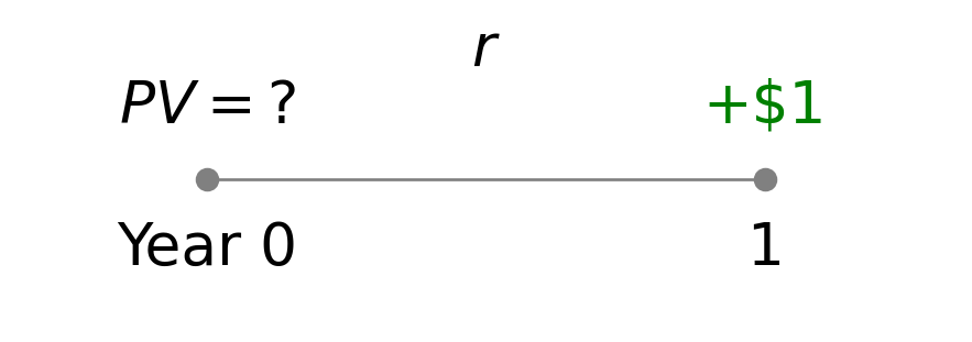
Consider a simple example of receiving $1 in one year. The present value (PV) of that future cash flow can be calculated using the formula:

\[ \text{Discount factor} = \frac{1}{1+r} = PV_0 \]

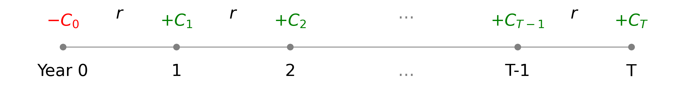
\[ \text{NPV}=C_0+C_1\left(\frac{1}{1+r}\right)+C_2\left(\frac{1}{1+r}\right)^2\ldots+C_{T-1}\left(\frac{1}{1+r}\right)^{T-1}+C_T\left(\frac{1}{1+r}\right)^T \]

What is the PV formula at time $t$? Can you simplify it to the NPV formula?

3.5 Net Present Value

Convert each future cash flow into present value
Use the formula, $C_t$ denotes cash flow in period t,

\[ PV_t = \frac{C_t}{(1+r)^t} \]

where $r$= the discount rate and $t$= time period (years).

Summing all present values gives the Net Present Value (NPV):

\[ NPV = C_0 + \sum_{t=1}^T \left(\frac{1}{1+r}\right)^tC_t \]

where $T$ = Total number of periods and $C_0$ = Initial investment.

Interpreting NPV Results

NPV	Interpretation	Suggested Action
> 0	The project is expected to generate more cash than it costs, indicating a profitable investment.	Consider proceeding with the project.
= 0	The project is expected to break even, generating CFs equal to the initial investment.	The project may be acceptable, but it does not create additional value.
< 0	The project is expected to generate less cash than it costs, indicating a loss.	Consider rejecting the project or re-evaluating assumptions.

Decision Rule

Conduct a scenario analysis to evaluate NPV under different assumptions (e.g., demand levels, cost fluctuations).
Prefer projects with higher positive NPV as they are expected to add more value to the company.

3.5.1 Example 1

Suppose you have a project requiring an initial investment of $200,000 (Year 0) with expected annual cash inflows over the next five years. Future cash inflows will be discounted at 10% to compute their present values.

Fill in the missing values in the table below to calculate the NPV of the project.
Evaluate whether the project is financially attractive based on the NPV result.

Year	Cash Flow	Discount Factor (10%)
0	-200,000
1	50,000
2	60,000
3	70,000
4	80,000
5	90,000
		NPV

To calculate the NPV, we first need to compute the discount factor for each year. Then, we can calculate the PV of each cash flow by multiplying the CF by its corresponding discount factor. Finally, we sum all the PVs to get the NPV.

Year	Cash Flow	Discount Factor (10%)	Present Value
0	-200,000	$(1.1)^0=1.0000$	-200,000
1	50,000	$(1.1)^{-1}=0.9091$	45,455
2	60,000	$(1.1)^{-2}=0.8264$	49,583
3	70,000	$(1.1)^{-3}=0.7513$	52,591
4	80,000	$(1.1)^{-4}=0.6830$	54,640
5	90,000	$(1.1)^{-5}=0.6209$	55,878
		NPV	$58,147

Since the NPV is positive, the project is expected to generate more cash than it costs, indicating a profitable investment. Therefore, the project is financially attractive and may be considered for implementation.

3.5.2 Example 2

For the cash flows of two options with $r = 0.1$ (10%), which option is better?

Year	Option 1	Option 2
0	-1,000,000	-1,400,000
1	300,000	400,000
2	300,000	400,000
3	300,000	400,000
4	300,000	400,000
5	300,000	400,000
	Option 1 NPV	Option 2 NPV

Fill in the missing values in the table to calculate the NPV of each option.
Evaluate which option is better based on the NPV results.

To calculate the NPV for each option, we will compute the present value of each cash flow using the formula $PV_t = C_t/(1+r)^t = C_t(1+r)^{-t}$, where $r = 0.1$ (10%). Then, we will sum the present values to get the NPV for each option.

Year	Option 1 PV	Option 2 PV
0	$-1,000,000(1.1)^0=-1,000,000$	$-1,400,000(1.1)^0=-1,400,000$
1	$300,000(1.1)^{-1}=272,727$	$400,000(1.1)^{-1}=363,636$
2	$300,000(1.1)^{-2}=247,934$	$400,000(1.1)^{-2}=330,579$
3	$300,000(1.1)^{-3}=225,394$	$400,000(1.1)^{-3}=300,526$
4	$300,000(1.1)^{-4}=204,904$	$400,000(1.1)^{-4}=273,205$
5	$300,000(1.1)^{-5}=186,276$	$400,000(1.1)^{-5}=248,369$
	Option 1 NPV $= 137,236$	Option 2 NPV $= 116,315$

Since the NPV of Option 1 is higher than that of Option 2, Option 1 is the better choice based on the NPV criterion.

3.5.3 Example 3: Target.com

Scenario

Estimated demand: 100,000 units for online orders
Required space: 1,000 sq. ft. for every 1,000 units
Revenue: $1.22 per unit of demand
Discount factor: 10% ($r = 0.1$)

TARGET

Questions

How much warehouse space should be leased in the next 3 years?
Should Target sign a 3-year lease contract or obtain warehousing space on the spot market each year?

Option 1: Spot Market

Spot market rate ~$1.20/sq.ft./year for each of the next 3 years

Option 2: 3-Year Lease Contract

Fixed lease rate of $1.00/sq.ft. locked in for 3 years

Option 1: Obtain space from the spot market each year

Spot market rate expected at $1.20/sq.ft./year for each of the next 3 years.
Required space 1,000 sq. ft. for every 1,000 units.
Estimated demand 100,000 units per year for online orders.
Revenue $1.22 for each unit of demand.

First, calculate the expected annual profit ($C_t$) if space is obtained from the spot market using discount factor $r = 0.1$ is given by

\[ \begin{aligned} \text{Profit} &= \text{Revenue} - \text{Expense} \\ &= (100{,}000 \text{ units} \times \$1.22) - (100{,}000 \text{ units} \times \$1.20) = \$2{,}000 \end{aligned} \]

Year	$C_t$	$PV_t$
0	2,000	2,000
1	2,000	1,818
2	2,000	1,653
	NPV	$5,471

\[ \begin{aligned} \text{NPV (no lease)} &= C_0 + \frac{C_1}{1+r} + \frac{C_2}{(1+r)^2} \\ &= 2{,}000 + \frac{2{,}000}{1.1} + \frac{2{,}000}{1.1^2} \\ \therefore \text{NPV (no lease)} &= \$5{,}471 \end{aligned} \]

Option 2: Sign a 3-year lease contract

100,000 sq.ft. of warehouse space are leased for the next 3 years.
Target pays $1 per sq.ft. of space leased each year.
Estimated demand 100,000 units per year for online orders.
Revenue $1.22 for each unit of demand.

Thus, the expected annual profit ($C_t$) is

\[ \text{Revenue} - \text{Expense} = 100{,}000 \times \$1.22 - 100{,}000 \times \$1.00 = \$22{,}000 \]

Year	$C_t$	$PV_t$
0	22,000	22,000
1	22,000	20,000
2	22,000	18,182
	NPV	$60,182

\[ \begin{aligned} \text{NPV (Lease)} &= C_0 + \frac{C_1}{1+r} + \frac{C_2}{(1+r)^2} \\ &= 22{,}000 + \frac{22{,}000}{1.1} + \frac{22{,}000}{1.1^2} \\ \therefore \text{NPV (Lease)} &= \$60{,}182 \end{aligned} \]

Comparing the NPV of Two Options

Year	$C_t$	$PV_t$
0	2,000	2,000
1	2,000	1,818
2	2,000	1,653
Option 1	NPV	$5,471

Year	$C_t$	$PV_t$
0	22,000	22,000
1	22,000	20,000
2	22,000	18,182
Option 2	NPV	$60,182

The NPV of signing the lease is 60,182 - 5,471 = $54,711 higher.
Assume that there is no uncertainty in the demand and costs, Target.com should go with Option 2.
However, if there is significant uncertainty in demand or costs, Target.com may want to consider the flexibility of the spot market despite its lower NPV.

How does uncertainty affect the decision between the two options? And how can we incorporate uncertainty into the NPV analysis?

3.6 Binomial Representation of Uncertainty

A binomial distribution is a discrete probability distribution that models the number of successes in a fixed number of independent trials of a binary experiment — where each trial results in only one of two outcomes: success or failure.

\[ P(X=k) = \binom{n}{k} p^k (1-p)^{n-k} \]

for $k=0,1,2,\dots,n$ and \[ \binom{n}{k} = \frac{n!}{k!(n-k)!} \]

Symbol	Description
$n$	Total number of trials
$k$	Number of successes
$p$	Probability of success on an individual trial
$1-p$	Probability of failure on an individual trial
$P(X=k)$	Probability of observing exactly $k$ successes in $n$ trials
$\dbinom{n}{k}$	The number of ways to choose $k$ successes from $n$ trials

Example: Binomial Representation of Demand Uncertainty

Suppose a company is launching a new product and wants to model the demand uncertainty using a binomial distribution.
The company estimates that there is a 60% chance that the product will be successful and a 40% chance that it will not be successful (failure).
The company plans to produce 100 units of the product.
What is the probability of observing exactly 70 units of demand?

From the question, identify the parameters:

\[ n=100, \quad k=70, \quad p=0.6 \]

The probability is calculated using the binomial formula:

\[ P(X=70) = \binom{100}{70} (0.6)^{70} (0.4)^{30} = \frac{100!}{70! \cdot 30!} (0.6)^{70} (0.4)^{30} = 0.01 \]

3.6.1 Multiplicative Binomial

Given a price $𝑃$ in Period 0, the possible outcomes in the future periods are

Period	Outcomes
0	$P$
1	$Pu,\; Pd$
2	$Pu^2,\; Pud,\; Pd^2$
3	$Pu^3,\; Pu^2d,\; Pud^2,\; Pd^3$
4	$Pu^4,\; Pu^3d,\; Pu^2d^2,\; Pud^3,\; Pd^4$

General formula for the price at time $t$ is

\[ Pu^t d^{T-t}, \quad t=0,1,2,\dots,T \]

At instant time $t=a$, the price can move to either

$Pu^{a+1}d^{T-a}$

with probability $\alpha$

$Pd^{a}u^{(T-a)+1}$

with probability $1-\alpha$

3.6.1 Multiplicative Binomial

%%{init: {
  "flowchart": {
    "padding": 30,
    "nodeSpacing": 30,
    "rankSpacing": 60
  },
  "themeVariables": {
    "fontSize": "22px"
  }
}}%%

flowchart LR
  P((P)) -->|α| Pu((Pu))
  P -->|1-α| Pd((Pd))

  Pu -->|α| Pu2((Pu²))
  Pu -->|1-α| Pud((Pud))
  Pd --> Pud
  Pd --> Pd2((Pd²))

  Pu2 -->|α| Pu3((Pu³))
  Pu2 -->|1-α| Pu2d((Pu²d))
  Pud --> Pu2d
  Pud --> Pud2((Pud²))
  Pd2 --> Pud2
  Pd2 --> Pd3((Pd³))

  Pu3 -->|α| Pu4((Pu⁴))
  Pu3 -->|1-α| Pu3d((Pu³d))
  Pu2d --> Pu3d
  Pu2d --> Pu2d2((Pu²d²))
  Pud2 --> Pu2d2
  Pud2 --> Pud3((Pud³))
  Pd3 --> Pud3
  Pd3 --> Pd4((Pd⁴))

  Pu4 -->|α| Pu5((Pu⁵))
  Pu4 -->|1-α| Pu4d((Pu⁴d))
  Pu3d --> Pu4d
  Pu3d --> Pu3d2((Pu³d²))
  Pu2d2 --> Pu3d2
  Pu2d2 --> Pu2d3((Pu²d³))
  Pud3 --> Pu2d3
  Pud3 --> Pud4((Pud⁴))
  Pd4 --> Pud4
  Pd4 --> Pd5((Pd⁵))

3.6.1 Multiplicative Binomial Examples

Example 1 Given:

Initial asset price P = 100
Up factor u = 1.2
Down factor d = 0.8

Construct the binomial price tree up to 3 periods.
List all possible outcomes at t = 3.
Express the general formula for price at any node.

%%{init: {
  "flowchart": {
    "htmlLabels": true,
    "padding": 40,
    "nodeSpacing": 15,
    "rankSpacing": 45
  },
  "theme": "base",
  "themeVariables": {
    "fontSize": "22px",
    "secondaryColor": "#ffffff",
    "secondaryTextColor": "#000000"
  }
}}%%

flowchart LR
  P([100]) --> Pu([120])
  P --> Pd([80])

  Pu --> Pu2([144])
  Pu --> Pud([96])
  Pd --> Pud
  Pd --> Pd2([64])

  Pu2 --> Pu3([172.8])
  Pu2 --> Pu2d([115.2])
  Pud --> Pu2d
  Pud --> Pud2([76.8])
  Pd2 --> Pud2
  Pd2 --> Pd3([51.2])

  classDef default fill:#ffffff,stroke:#000000,color:#000000;

The general formula for price at any node is given by

\[ P u^t d^{T-t} = 100(1.2)^t (0.8)^{T-t}, \]

\[ \quad t=0,1,2,\dots,T \]

where $t$ is the number of up moves and $T-t$ is the number of down moves.

3.6.1 Multiplicative Binomial Examples

Example 2 Given:

Initial asset price P = 50
u = 1.1, d = 0.9
Risk-neutral probability $\alpha$ = 0.6

Calculate all possible prices at T = 2.
Find the probability of ending up at each price level.
What is the probability that the final price is greater than 50?

%%{init: {
  "flowchart": {
    "htmlLabels": true,
    "padding": 40,
    "nodeSpacing": 15,
    "rankSpacing": 45
  },
  "theme": "base",
  "themeVariables": {
    "fontSize": "22px",
    "secondaryColor": "#ffffff",
    "secondaryTextColor": "#000000"
  }
}}%%

flowchart LR
  P([50]) -->|α|Pu([55])
  P -->|1-α| Pd([45])

  Pu -->|α| Pu2([60.5])
  Pu -->|1-α| Pud([49.5])
  Pd -->|α| Pud
  Pd -->|1-α| Pd2([40.5])

  classDef default fill:#ffffff,stroke:#000000,color:#000000;

$P=\alpha^2=0.36=P(\text{Final price} > 50)$

$P=\alpha(1-\alpha)=0.24$

$P=(1-\alpha)^2=0.16$

3.6.2 Additive Binomial

Given a price $𝑃$ in Period 0, the possible outcomes in the future periods are

Period	Value
0	$P$
1	$P+u,\; P-d$
2	$P+2u,\; P+u-d,\; P-2d$
3	$P+3u,\; P+2u-d,\; P+u-2d,\; P-3d$
4	$P+4u,\; P+3u-d,\; P+2u-2d,\; P+u-3d,\; P-4d$

General formula for the price at time $t$ is

\[ P + tu - (T-t)d, \quad t=0,1,2,\dots,T \]

3.6.2 Additive Binomial

%%{init: {
  "flowchart": {
    "padding": 30,
    "nodeSpacing": 40,
    "rankSpacing": 40
  },
  "themeVariables": {
    "fontSize": "22px"
  }
}}%%

flowchart LR
  P([P]) -->|α| Pu([P+u])
  P -->|1-α| Pd([P-d])

  Pu -->|α| Pu2([P+2u])
  Pu -->|1-α| Pud([P+u-d])
  Pd --> Pud
  Pd --> Pd2([P-2d])

  Pu2 -->|α| Pu3([P+3u])
  Pu2 -->|1-α| Pu2d([P+2u-d])
  Pud --> Pu2d
  Pud --> Pud2([P+u-2d])
  Pd2 --> Pud2
  Pd2 --> Pd3([P-3d])

  Pu3 -->|α| Pu4([P+4u])
  Pu3 -->|1-α| Pu3d([P+3u-d])
  Pu2d --> Pu3d
  Pu2d --> Pu2d2([P+2u-2d])
  Pud2 --> Pu2d2
  Pud2 --> Pud3([P+u-3d])
  Pd3 --> Pud3
  Pd3 --> Pd4([P-4d])

  Pu4 -->|α| Pu5([P+5u])
  Pu4 -->|1-α| Pu4d([P+4u-d])
  Pu3d --> Pu4d
  Pu3d --> Pu3d2([P+3u-2d])
  Pu2d2 --> Pu3d2
  Pu2d2 --> Pu2d3([P+2u-3d])
  Pud3 --> Pu2d3
  Pud3 --> Pud4([P+u-4d])
  Pd4 --> Pud4
  Pd4 --> Pd5([P-5d])

3.6.2 Additive Binomial Examples

Example 1 Given:

Initial asset price P = 50
Up increment u = 3
Down decrement d = 2

Construct the additive binomial price tree for T = 3.
List all possible outcomes at T = 3.
Express the general formula for price at any node.

%%{init: {
  "flowchart": {
    "htmlLabels": true,
    "padding": 35,
    "nodeSpacing": 15,
    "rankSpacing": 40
  },
  "theme": "base",
  "themeVariables": {
    "fontSize": "22px",
    "secondaryColor": "#ffffff",
    "secondaryTextColor": "#000000"
  }
}}%%

flowchart LR
  P((50)) -->|α|Pu((53))
  P -->|1-α| Pd((48))

  Pu -->|α| Pu2((56))
  Pu -->|1-α| Pud((51))
  Pd -->|α| Pud
  Pd -->|1-α| Pd2((46))

  classDef default fill:#ffffff,stroke:#000000,color:#000000;

The general formula for price at any node is given by

\[ \begin{aligned} P + tu - (T-t)d &= 50 + 3t - 2(T-t) \\ &= 50 + 5t - 2T, \end{aligned} \]

\[ \quad t=0,1,2,3, \dots,T \]

where $t$ is the number of up moves and $T-t$ is the number of down moves.

3.6.2 Additive Binomial Examples

Example 2 Using the same parameters: P = 100 and T = 2,

Build both the additive and multiplicative trees and compare the final prices.
For additive model, u = 5 and d = 3. For multiplicative model, u = +5%, d = -3%
Discuss which model may be more realistic in financial contexts and why.

Additive Tree

%%{init: {
  "flowchart": {
    "htmlLabels": true,
    "padding": 25,
    "nodeSpacing": 15,
    "rankSpacing": 45
  },
  "theme": "base",
  "themeVariables": {
    "fontSize": "22px",
    "secondaryColor": "#ffffff",
    "secondaryTextColor": "#000000"
  }
}}%%

flowchart LR
  P([100]) -->|α|Pu([105])
  P -->|1-α| Pd([97])

  Pu -->|α| Pu2([110])
  Pu -->|1-α| Pud([102])
  Pd -->|α| Pud
  Pd -->|1-α| Pd2([94])

  classDef default fill:#fff3cd,stroke:#000000,color:#000000;

Multiplicative Tree

%%{init: {
  "flowchart": {
    "htmlLabels": true,
    "padding": 25,
    "nodeSpacing": 15,
    "rankSpacing": 45
  },
  "theme": "base",
  "themeVariables": {
    "fontSize": "22px",
    "secondaryColor": "#ffffff",
    "secondaryTextColor": "#000000"
  }
}}%%

flowchart LR
  P([100]) -->|α|Pu([105])
  P -->|1-α| Pd([97])

  Pu -->|α| Pu2([110.25])
  Pu -->|1-α| Pud([101.85])
  Pd -->|α| Pud
  Pd -->|1-α| Pd2([94.09])

  classDef default fill:#f8d7da,stroke:#000000,color:#000000;

The multiplicative model may be more realistic in financial contexts because it captures the compounding effect of returns.

4. Decision Trees

A decision tree is a decision support recursive partitioning structure that uses a tree-like model of decisions and their possible consequences, including chance event outcomes, resource costs, and utility.

Binomial Tree

Each node has two outcomes: up or down: (binary branching)

%%{init: {
  "flowchart": {
    "padding": 20,
    "nodeSpacing": 5,
    "rankSpacing": 70
  },
  "themeVariables": {
    "fontSize": "22px"
  }
}}%%

flowchart LR
  P(( )) --> Pu(( ))
  P --> Pd(( ))

  Pu --> Pu2(( ))
  Pu --> Pud(( ))
  Pd --> Pud
  Pd --> Pd2(( ))

  Pu2 --> Pu3(( ))
  Pu2 --> Pu2d(( ))
  Pud --> Pu2d
  Pud --> Pud2(( ))
  Pd2 --> Pud2
  Pd2 --> Pd3(( ))

  Pu3 --> Pu4(( ))
  Pu3 --> Pu3d(( ))
  Pu2d --> Pu3d(( ))
  Pu2d --> Pu2d2(( ))
  Pud2 --> Pu2d2(( ))
  Pud2 --> Pud3(( ))
  Pd3 --> Pud3
  Pd3 --> Pd4(( ))

  classDef default fill:#cfe2ff,stroke:#000000,color:#ffffff;

Move forward in discrete time steps

Based on risk-neutral probabilities

Decision Tree

Each node can have multiple branches representing choices or events

%%{init: {
  "flowchart": {
    "padding": 22,
    "nodeSpacing": 8,
    "rankSpacing": 70
  },
  "themeVariables": {
    "fontSize": "22px"
  }
}}%%

flowchart LR
  P0(( )) --> P11(( ))
  P0 --> P12(( ))
  P0 --> P13(( ))

  P11 --> P21(( ))
  P11 --> P22(( ))
  
  P12 --> P22
  P12 --> P23(( ))
  P12 --> P24(( ))
  P12 --> P25(( ))

  P21 --> P31(( ))

  P22 --> P31
  P22 --> P32(( ))

  P23 --> P32
  P23 --> P33(( ))
  P23 --> P34(( ))

  P31 --> P41(( ))
  P31 --> P42(( ))

  P33 --> P43(( ))

  P34 --> P43(( ))
  P34 --> P44(( ))


  classDef default fill:#d1e7dd,stroke:#000000,color:#ffffff;

Move along decision-event-decision cycles

Includes probabilities and payoffs

4.1.1 Example 1: Warehouse Location Decision

A company must decide how to expand its distribution network.

Decision Node

Choose between two strategies:

Build a Large DC Now

Build a Small DC with Option to Expand Later

Chance Node: Future Demand

Demand next year is uncertain:

High Demand (Probability = 0.6)

Low Demand (Probability = 0.4)

%%{init: {
  "flowchart": {
    "htmlLabels": true,
    "padding": 40,
    "nodeSpacing": 5,
    "rankSpacing": 80
  },
  "theme": "base",
  "themeVariables": {
    "fontSize": "20px",
    "secondaryColor": "#ffffff"
  }
}}%%

graph LR
    A(["Decision"])

    A --> B(["Large DC"])
    A --> C(["Small DC"])

    B -->|0.6| B1(["High Demand<br/>NPV = $12M"])
    B -->|0.4| B2(["Low Demand<br/>NPV = $2M"])

    C -->|0.6| C1(["High Demand<br/>NPV = $15M"])
    C -->|0.4| C2(["Low Demand<br/>NPV = $4M"])

    classDef default fill:#d1e7dd,stroke:#000000,color:#000000;

\[ EV_{Large} = 0.6(12) + 0.4(2) = \$8\text{M} \]

\[ EV_{Flexible} = 0.6(15) + 0.4(4) = \$10.6\text{M} \]

The flexible strategy is preferred because it provides a higher expected value and allows adaptation to demand uncertainty.

4.1.2 Example 2: Regional Distribution Hub Decision

A logistics company must decide whether to build a central hub or keep decentralised warehouses.

Decision Node

Two alternatives:

Build a Central DC

Keep Current Decentralised Warehouses

Chance Node

Demand over the next 5 years is uncertain:

High Growth (Probability = 0.5)

Moderate Growth (Probability = 0.3)

Low Growth (Probability = 0.2)

%%{init: {
  "flowchart": {
    "htmlLabels": true,
    "padding": 30,
    "nodeSpacing": 5,
    "rankSpacing": 160
  },
  "theme": "base",
  "themeVariables": {
    "fontSize": "20px",
    "secondaryColor": "#ffffff"
  }
}}%%
flowchart LR

  A(["Decision"])

  A --> B(["Central Hub"])
  A --> C(["Decentralised"])

  B -->|0.5| B1(["$25M"])
  B -->|0.3| B2(["$14M"])
  B -->|0.2| B3(["-$5M"])

  C -->|0.5| C1(["$18M"])
  C -->|0.3| C2(["$12M"])
  C -->|0.2| C3(["$6M"])

  classDef default fill:#fff3cd,stroke:#000000,color:#000000;

\[ EV_\text{Central Hub} = 0.5(25) + 0.3(14) + 0.2(-5) = 12.5 + 4.2 - 1 = 15.7 \]

\[ EV_\text{Decentralised} = 0.5(18) + 0.3(12) + 0.2(6) = 9 + 3.6 + 1.2 = 13.8 \]

The central hub strategy has the higher expected value (15.7M) and is the preferred network design decision.

4.2 Evaluating NPV: Bellman’s Principle

Solve the problem from the end (future outcomes) back to the beginning.

Structure the decision tree
- Draw nodes and terminal nodes (outcomes) connected with arrows
Assign payoffs and probabilities for each node
- For each node, calculate payoffs (or a combination of demand and price) and state the probability.
Work backwards (Bellman’s principle)
- From the terminal node, calculate
  
  $\text{Expected Monetary Value (EMV)} = \sum (\text{Probability} \times \text{Payoff})$
- Discount EMV to Present Value (PV)
Continue working backward until you reach the initial decision.

4.2.1 Example 1: Project Evaluation (1 Period)

Imagine a company considering a project that costs $50,000. There are two scenarios:

High demand (60%): earns $100,000
Low demand (40%): earns $30,000

Assume a discount rate of 10% and 1-year horizon. Evaluate the project.

Starts from the terminal node,

\[ \begin{aligned} EMV &= 0.6(100,000)+0.4(30,000)=60,000+12,000=72,000 \\[.5em] PV &= 72,000 / 1.1 = 65,455 \\[.5em] NPV &= PV - C_0 = 65,455 - 50,000 = \textbf{\$15,455} > 0 \end{aligned} \]

Positive NPV suggests a profitable investment in 1-year horizon.

4.2.2 Example 2: Project Evaluation (2 Periods)

Imagine a company considering a project that costs $50,000.

In Year 1,

High demand (60%): the company can invest $20,000 more to expand.
Low demand (40%): the project ends; no further payoff.

In Year 2, expansion leads to:

$150,000 (70%)
$50,000 (30%)

Note. For this example, the cashflows are realised at Year 2.

Use the discount rate of 10%.

Draw a Decision Tree
Calculate the NPV of the project

%%{init: {
  "flowchart": {
    "htmlLabels": true,
    "padding": 20,
    "nodeSpacing": 30,
    "rankSpacing": 40
  },
  "theme": "default",
  "themeVariables": {
    "fontSize": "20px",
    "secondaryColor": "#ffffff"
  }
}}%%
flowchart LR
  subgraph P0["Year 0"]
  A([-$50k])
  end

  subgraph P1["Year 1"]
  A -->|0.6| B([High<br>-$20k])
  A -->|0.4| C([Low])
  end

  subgraph P2["Year 2"]
  B -->|0.7| D([$150k])
  B -->|0.3| E([$50k])
  end

  classDef default fill:#cfe2ff,stroke:#000000,color:#000000;
  style B color:green;
  style P0 fill:#ffffff,stroke:#ffffff
  style P1 fill:#ffffff,stroke:#ffffff
  style P2 fill:#ffffff,stroke:#ffffff

$\text{Year 2}$: $EMV_\text{Year 2}$ → $PV_\text{Year 1}$ → $\text{Net Payoff}_\text{Year 1}$

\[ EMV_\text{Year 2} = 0.7(150,000) + 0.3(50,000) = 105,000 + 15,000 = 120,000 \]

\[ PV_\text{Year 1} = 120,000 / 1.1 = 109,091 \]

\[ \text{Net payoff at Year 1} = 109,091 - \color{green}{20,000} = \color{purple}{89,091} \]

$\text{Year 1}$: $EMV_\text{Year 1}$ → $PV_\text{Year 0}$ → $\text{Net Payoff}_\text{Year 0}$

\[ EMV_\text{Year 1} = 0.6(\color{purple}{89,091}) + 0.4(0) = 53,455 \]

\[ PV_\text{Year 0} = 53,455 / 1.1 = 48,595 \]

\[ NPV_\text{Year 0} = PV_\text{Year 0} - C_0 = 48,595 - 50,000 = \textbf{-\$1,405} \]

4.2.3 Example 3: Multi-Stage Project Evaluation

Imagine a company considering a project that costs $50,000.

In Year 1,

High demand (60%):
- Earns $30,000 immediately
- The company can invest $20,000 more to expand.
Low demand (40%):
- Earns $10,000 immediately
- The project terminates.

In Year 2, expansion leads to: $150,000 (70%) or $50,000 (30%)

Use the discount rate of 10%.

Draw a Decision Tree
Calculate the NPV of the project

%%{init: {
  "flowchart": {
    "htmlLabels": true,
    "padding": 20,
    "nodeSpacing": 30,
    "rankSpacing": 50
  },
  "theme": "base",
  "themeVariables": {
    "fontSize": "20px",
    "secondaryColor": "#ffffff"
  }
}}%%
flowchart LR
  subgraph P0["Year 0"]
  A([-$50k])
  end

  subgraph P1["Year 1"]
  A -->|0.6| B([$30k<br>-$20k])
  A -->|0.4| C([$10k])
  end

  subgraph P2["Year 2"]
  B -->|0.7| D([$150k])
  B -->|0.3| E([$50k])
  end

  classDef default fill:#d1e7dd,stroke:#00000,color:#000000;
  style C color:red;
  style B color:green;
  style P0 fill:#ffffff,stroke:#ffffff
  style P1 fill:#ffffff,stroke:#ffffff
  style P2 fill:#ffffff,stroke:#ffffff

$\text{Year 2}$: $EMV_\text{Year 2}$ → $PV_\text{Year 1}$ → $\text{Net Payoff}_\text{Year 1}$

\[ EMV_\text{Year 2} = 0.7(150,000) + 0.3(50,000) = 105,000 + 15,000 = 120,000 \]

\[ PV_\text{Year 1} = 120,000 / 1.1 = 109,091 \]

\[ \text{Net payoff at Year 1} = 109,091 \color{green}{- 20,000 + 30,000}= \color{purple}{119,091} \]

$\text{Year 1}$: $EMV_\text{Year 1}$ → $PV_\text{Year 0}$ → $\text{Net Payoff}_\text{Year 0}$

\[ EMV_\text{Year 1} = 0.6(\color{purple}{119,091}) + 0.4(\color{red}{10,000}) = 75,455 \]

\[ PV_\text{Year 0} = 75,455 / 1.1 = 68,595 \]

\[ NPV_\text{Year 0} = PV_\text{Year 0} - C_0 = 68,595 - 50,000 = \textbf{\$18,595} \]

4.2.4 Example 4: Target.com

Let’s revisit 3.5.3 Example 3 – Target.com.

The Target manager anticipated uncertainty in demand and spot prices over the next three years

❖ Long-term lease
- ✓ Cheaper than the spot market rate
- ✓ Could go unused if demand is lower than forecast
❖ Spot market
- ✓ Currently high, but future rates could decrease.
- ✓ Cost a lot if future demand is higher than expected.
❖ Decide whether to
- ✓ Lease warehouse space for the coming years and
- ✓ The quantity to lease

Identify all options and information

Option 1:

Option 2:

Option 3:

Get all warehousing space from the spot market as needed.

Sign a three-year lease for a fixed amount of warehouse space and get additional requirements from the spot market.

Sign a flexible lease with a minimum charge that allows variable usage of warehouse space up to a limit with additional requirement from the spot market.

r = 10%
Revenue = $1.22/unit
Lease price = $1/sq.ft/year
1000 sq.ft is required for every 1000 units of demand
Demand (D) = 100,000 units/year can go up/down by 20% with equal probability
Spot market price (P) = $1.2/sq.ft/year can go up/down by 10% with equal probability
Prices of warehouse space and demand for product fluctuate independently; thus, 𝑃(𝐴∩𝐵)=𝑃(𝐴)𝑃(𝐵).

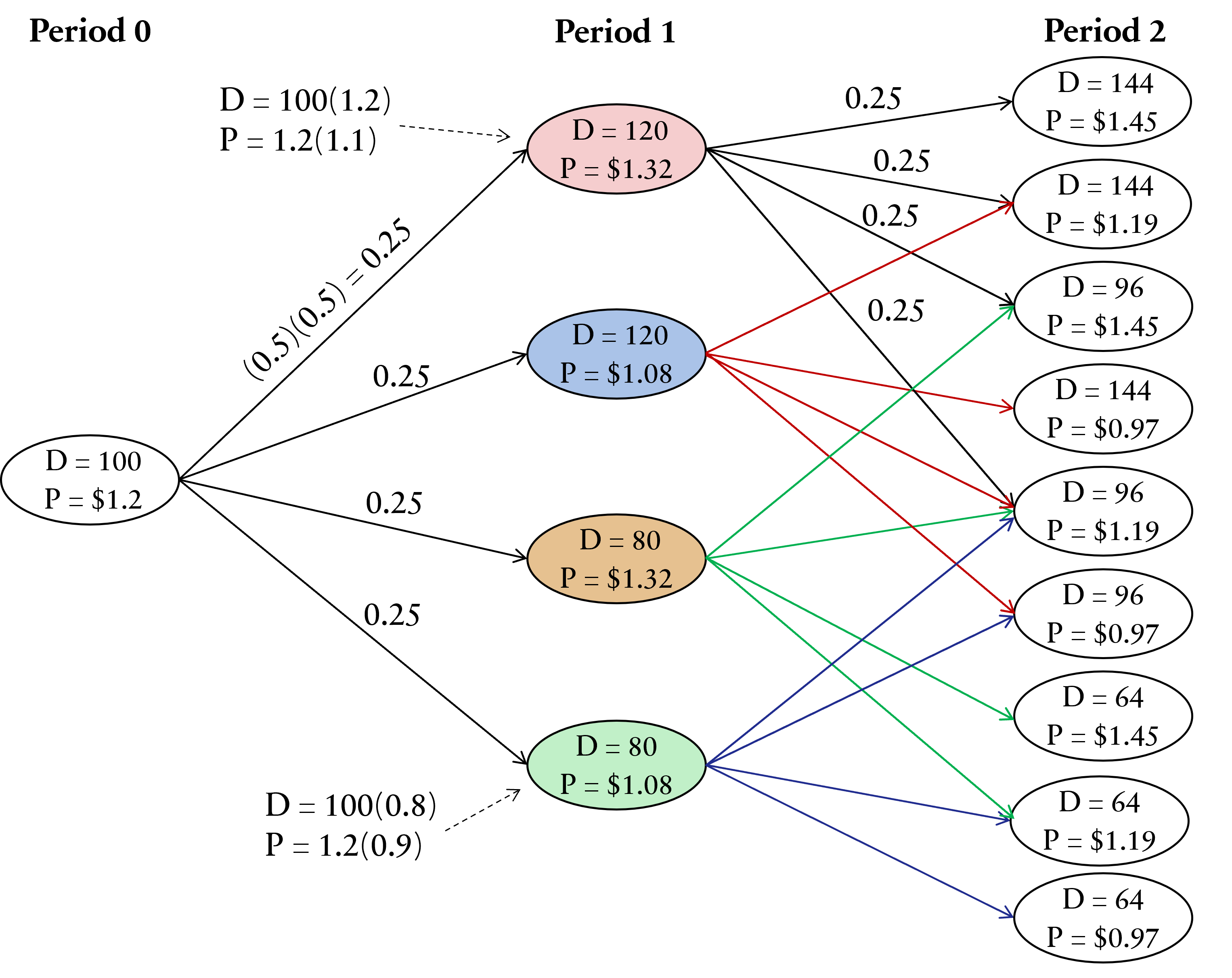
Construct the decision tree for demand and spot price uncertainty (Period 0 → Period 1)

%%{init: {
  "flowchart": {
    "htmlLabels": true,
    "padding": 15,
    "nodeSpacing": 15,
    "rankSpacing": 100
  },
  "theme": "base",
  "themeVariables": {
    "fontSize": "22px",
    "secondaryColor": "#ffffff",
  }
}}%%

flowchart LR

%% ----- Period 0 -----
subgraph P0["Period 0"]
A["D=100k<br/>p=$1.2"]
end

%% ----- Period 1 -----
subgraph P1["Period 1"]
B["D = 100(1.2) = 120<br/><br/> P = 1.2(1.1) = $1.32"]
C["D = _________________<br/><br/> P = _________________"]
D["D = _________________<br/><br/> P = _________________"]
E["D = _________________<br/><br/> P = _________________"]
end



%% Transitions
A -->|"(0.5)(0.5)=0.25"| B
A -->|0.25| C
A -->|0.25| D
A -->|0.25| E




%% Subgraph background (white)
style P0 fill:#ffffff,stroke:#ffffff
style P1 fill:#ffffff,stroke:#ffffff

style A fill:#ffffff;
style B fill:#f8d7da;
style C fill:#cfe2ff,color:#cfe2ff;
style D fill:#fff3cd,color:#fff3cd;
style E fill:#d1e7dd,color:#d1e7dd;
  
classDef default stroke:#000000,color:#000000;

Construct the decision tree for demand and spot price uncertainty (Period 0 → Period 1)

%%{init: {
  "flowchart": {
    "htmlLabels": true,
    "padding": 15,
    "nodeSpacing": 25,
    "rankSpacing": 100
  },
  "theme": "base",
  "themeVariables": {
    "fontSize": "22px",
    "secondaryColor": "#ffffff",
  }
}}%%

flowchart LR

%% ----- Period 0 -----
subgraph P0["Period 0"]
A["D=100k<br/>p=$1.2"]
end

%% ----- Period 1 -----
subgraph P1["Period 1"]
B["D = 120<br/>P = $1.32"]
C["D = 120<br/>P = $1.08"]
D["D = 80<br/>P = $1.32"]
E["D = 80<br/>P = $1.08"]
end



%% Transitions
A -->|"0.25"| B
A -->|0.25| C
A -->|0.25| D
A -->|0.25| E




%% Subgraph background (white)
style P0 fill:#ffffff,stroke:#ffffff
style P1 fill:#ffffff,stroke:#ffffff

style A fill:#ffffff;
style B fill:#f8d7da;
style C fill:#cfe2ff;
style D fill:#fff3cd;
style E fill:#d1e7dd;
  
classDef default stroke:#000000,color:#000000;

Construct the decision tree for demand and spot price uncertainty (Period 1 → Period 2)

%%{init: {
  "flowchart": {
    "htmlLabels": true,
    "padding": 15,
    "nodeSpacing": 50,
    "rankSpacing": 200
  },
  "theme": "base",
  "themeVariables": {
    "fontSize": "22px",
    "secondaryColor": "#ffffff",
  }
}}%%

flowchart LR

%% ----- Period 0 -----
subgraph P0["Period 0"]
A["D=100k<br/>p=$1.2"]
end

%% ----- Period 1 -----
subgraph P1["Period 1"]
B["D = 120<br/>P = $1.32"]
C[" "]
D[" "]
E[" "]
end

%% ----- Period 2 -----
subgraph P2["Period 2"]
F["D = ______________<br/>P = ______________"]
G["D = ______________<br/>P = ______________"]
H["D = ______________<br/>P = ______________"]
I["D = ______________<br/>P = ______________"]
end

%% Transitions
A -->|"0.25"| B
A -->|0.25| C
A -->|0.25| D
A -->|0.25| E

B -->|0.25| F
B -->|0.25| G
B -->|0.25| H
B -->|0.25| I

%% Subgraph background (white)
style P0 fill:#ffffff,stroke:#ffffff
style P1 fill:#ffffff,stroke:#ffffff
style P2 fill:#ffffff,stroke:#ffffff

style B fill:#f8d7da;
style C fill:#cfe2ff,color:#cfe2ff;
style D fill:#fff3cd,color:#fff3cd;
style E fill:#d1e7dd,color:#d1e7dd;
style F color:#ffffff;
style G color:#ffffff;
style H color:#ffffff;
style I color:#ffffff;
  
classDef default stroke:#000000,color:#000000, fill:#ffffff;

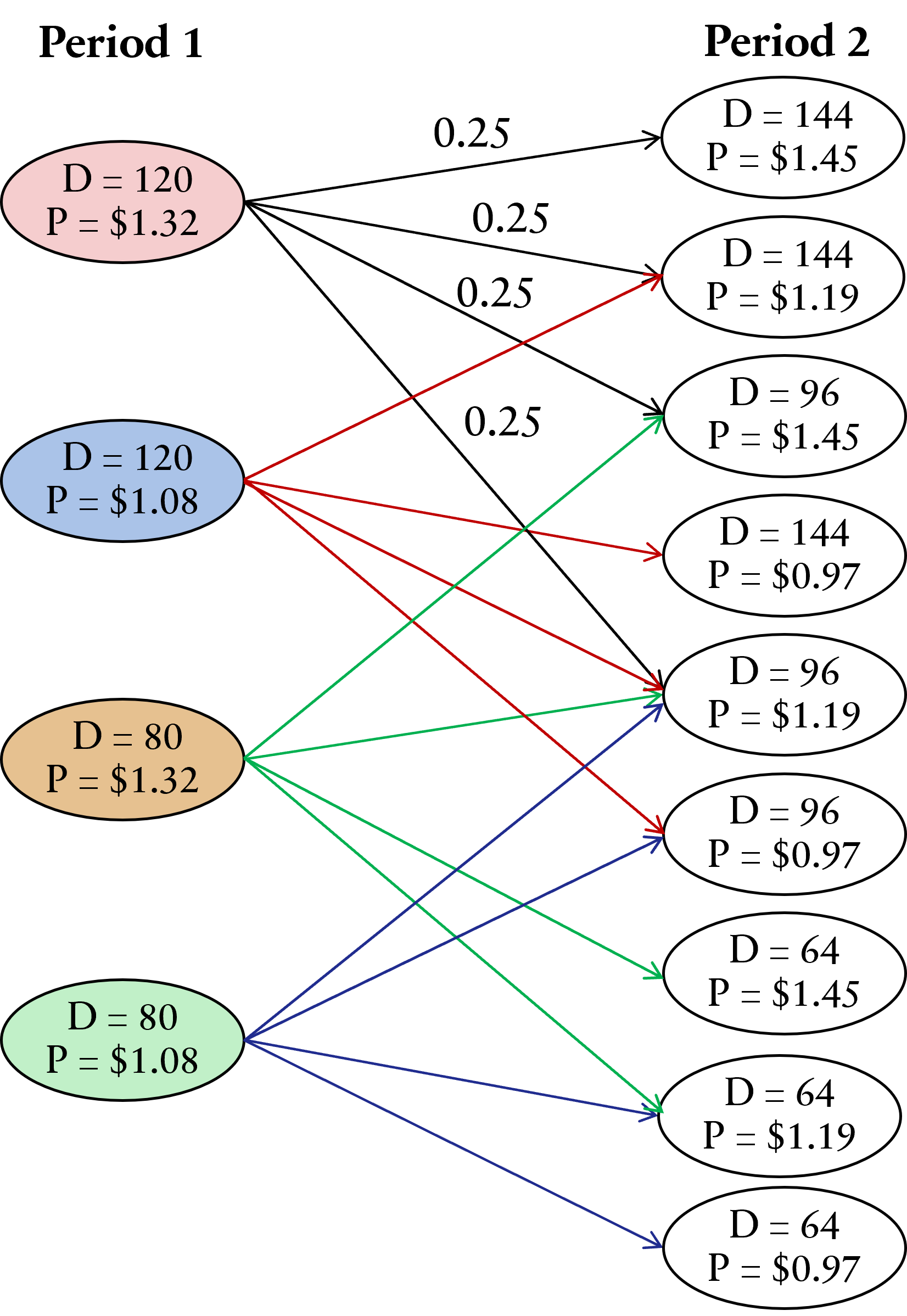
Construct the decision tree for demand and spot price uncertainty (Period 1 → Period 2)

%%{init: {
  "flowchart": {
    "htmlLabels": true,
    "padding": 15,
    "nodeSpacing": 50,
    "rankSpacing": 200
  },
  "theme": "base",
  "themeVariables": {
    "fontSize": "22px",
    "secondaryColor": "#ffffff",
  }
}}%%

flowchart LR

%% ----- Period 0 -----
subgraph P0["Period 0"]
A["D=100k<br/>p=$1.2"]
end

%% ----- Period 1 -----
subgraph P1["Period 1"]
B["D = 120<br/>P = $1.32"]
C[" "]
D[" "]
E[" "]
end

%% ----- Period 2 -----
subgraph P2["Period 2"]
F["D = 144<br/>P = $1.45"]
G["D = 144<br/>P = $1.19"]
H["D = 96<br/>P = $1.45"]
I["D = 96<br/>P = $0.97"]
end

%% Transitions
A -->|"0.25"| B
A -->|0.25| C
A -->|0.25| D
A -->|0.25| E

B -->|0.25| F
B -->|0.25| G
B -->|0.25| H
B -->|0.25| I

%% Subgraph background (white)
style P0 fill:#ffffff,stroke:#ffffff
style P1 fill:#ffffff,stroke:#ffffff
style P2 fill:#ffffff,stroke:#ffffff

style B fill:#f8d7da;
style C fill:#cfe2ff,color:#cfe2ff;
style D fill:#fff3cd,color:#fff3cd;
style E fill:#d1e7dd,color:#d1e7dd;
  
classDef default stroke:#000000,color:#000000, fill:#ffffff;

Construct the decision tree for demand and spot price uncertainty for two periods

Option 1: Get all warehousing space from the spot market as needed.

Calculate payoff at Period 2

Table 1. Profit (payoff) at Period 2 for Option 1 in 1000s.
Demand (D)	Spot Price (P)	Revenue (1.22 x D)	Cost (D × P)	Profit (R - C)
144	1.45	175.68	208.80	-33.12
144	1.19	175.68	171.36	4.32
144	0.97	175.68	139.68	36.00
96	1.45	117.12	139.20	-22.08
96	1.19	117.12	114.24	2.88
96	0.97	117.12	93.12	24.00
64	1.45	78.08	92.80	-14.72
64	1.19	78.08	76.16	1.92
64	0.97	78.08	62.08	16.00

Calculate $EMV_2$ for each node at Period 1, where $EMV_2 = \sum(\text{Probability} \times \text{Profit}_2)$

Table 2. Expected value (EV) of Each Terminal Node
D	P	Profit	EV
144	1.45	-33.12	-8.28
144	1.19	4.32	1.08
144	0.97	36.00	9.00
96	1.45	-22.08	-5.52
96	1.19	2.88	0.72
96	0.97	24.00	6.00
64	1.45	-14.72	-3.68
64	1.19	1.92	0.48
64	0.97	16.00	4.00

For each terminal node, calculate EV.
Sum the corresponding EVs to get $EMV_2$.
Example. Red Node $(D = 120, P = \$1.32)$:

%%{init:{'flowchart':{'nodeSpacing': 10, 'rankSpacing': 40}}}%%
flowchart LR

subgraph P1["Period 1"]
A["D=120<br/>p=$1.32"]
end

subgraph P2["Period 2"]
B["D=144<br/>p=$1.45"]
C["D=144<br/>p=$1.19"]
D["D=96<br/>p=$1.45"]
E["D=96<br/>p=$1.19"]
end

A -->|0.25| B
A -->|0.25| C
A -->|0.25| D
A -->|0.25| E

B --> F(["Profit = -33.12<br/>EV = 0.25x-33.12 = -8.28"])
C --> G(["Profit = 4.32<br/>EV = 0.25x4.32 = 1.08"])
D --> H(["Profit = -22.08<br/>EV = 0.25x-22.08 = -5.52"])
E --> I(["Profit = 2.88<br/>EV = 0.25x2.88 = 0.72"])


style P1 fill:#ffffff,stroke:#ffffff
style P2 fill:#ffffff,stroke:#ffffff

style A fill:#f8d7da;
style B fill:#ffffff;
style C fill:#ffffff;
style D fill:#ffffff;
style E fill:#ffffff;
style F fill:#ffffff,stroke:#ffffff;
style G fill:#ffffff,stroke:#ffffff;
style H fill:#ffffff,stroke:#ffffff;
style I fill:#ffffff,stroke:#ffffff;

linkStyle default stroke:#000,stroke-width:2px

Red Node: $EMV_2$ = -8.28 + 1.08 - 5.52 + 0.72 = -12.00

Exercise: Calculate $EMV_2$ for the blue node $(D = 120, P = \$1.08)$.

Table 3. Expected value (EV) at Period 2 for Each Terminal Node
D	P	Profit	EV
144	1.45	-33.12	-8.28
144	1.19	4.32	1.08
144	0.97	36.00	9.00
96	1.45	-22.08	-5.52
96	1.19	2.88	0.72
96	0.97	24.00	6.00
64	1.45	-14.72	-3.68
64	1.19	1.92	0.48
64	0.97	16.00	4.00

%%{init:{'flowchart':{'nodeSpacing': 15, 'rankSpacing': 40, 'curve': 'basis', 'layout': 'elk'}}}%%
flowchart LR

subgraph P1["Period 1"]
A["D=120<br/>p=$1.08"]
end

subgraph P2["Period 2"]
B["D=144<br/>p=$1.19"]
C["D=144<br/>p=$0.97"]
D["D=96<br/>p=$1.19"]
E["D=96<br/>p=$0.97"]
end

A -->|0.25| B
A -->|0.25| C
A -->|0.25| D
A -->|0.25| E

B --> F([" "])
C --> G([" "])
D --> H([" "])
E --> I([" "])

style P1 fill:#ffffff,stroke:#ffffff
style P2 fill:#ffffff,stroke:#ffffff

style B fill:#ffffff;
style C fill:#ffffff;
style D fill:#ffffff;
style E fill:#ffffff;
style F fill:#ffffff,stroke:#ffffff;
style G fill:#ffffff,stroke:#ffffff;
style H fill:#ffffff,stroke:#ffffff;
style I fill:#ffffff,stroke:#ffffff;

linkStyle default stroke:#000,stroke-width:2px

Blue Node $EMV_2$ =

Yellow Node $EMV_2$ =

Green Node $EMV_2$ =

Calculate Total EMV at Period 1

P1 Nodes $\;\;$ Step 2 $\quad$ /1.1 $\;\;$ 1.22 x D $\;\;$ D x P $\;\;$ Payoff $\;$ x0.25

D	P	$EMV_2$	$PV_1$	Revenue	Cost	Profit	EV
120	1.32	-12.00	-10.91	146.40	158.40	-22.91	-5.73
120	1.08	16.80	15.27	146.40	129.60	32.07	8.02
80	1.32	-8.00	-7.27	97.60	105.60	-15.27	-3.82
80	1.08	11.20	10.18	101.82	86.40	21.38	5.35

\[ EMV_\text{Period 1} = -5.73 + 8.02 - 3.82 + 5.35 = \textbf{3.82} \]

Calculate NPV

P0 Node $\;\;$ Step 3 $\quad$ /1.1 $\;\;$ 1.22 x D $\;\;$ D x P $\;\;$ NPV

D	P	$EMV_1$	$PV_0$	Revenue	Cost	Profit
100	1.20	3.82	3.47	122.00	120.00	5.47

The NPV for option 1 is $5,471.07 (if calculate exactly up to 2 decimal places)

Option 2: Sign a 3-year lease for 100,000 sq.ft. for $1/sq.ft. and obtain extra on spot market if needed.

Calculate payoff at Period 2

The total cost for this option is 100k lease + extra warehouse cost.

\[ \text{Cost} = 100 + \text{max}(0, D - 100) \times P \quad \text{(in 1000s)} \]

D	P	Revenue	Cost	Profit
144	1.45	175.68	163.80	11.88
144	1.19	175.68	152.36	23.32
144	0.97	175.68	142.68	33.00
96	1.45	117.12	100.00	17.12
96	1.19	117.12	100.00	17.12
96	0.97	117.12	100.00	17.12
64	1.45	78.08	100.00	-21.92
64	1.19	78.08	100.00	-21.92
64	0.97	78.08	100.00	-21.92

Calculate $EMV_2$ for each node at Period 1

For each terminal node, calculate EV.
Sum the corresponding EVs to get EMV for each node at Period 1.

D	P	Profit (Payoff)	EV = Payoff x 0.25
144	1.45	11.88	2.97
144	1.19	23.32	5.83
144	0.97	33.00	8.25
96	1.45	17.12	4.28
96	1.19	17.12	4.28
96	0.97	17.12	4.28
64	1.45	-21.92	-5.48
64	1.19	-21.92	-5.48
64	0.97	-21.92	-5.48

Red Node $EMV_2$ = 2.97 + 5.83 + 4.28 + 4.28 = 17.36
Blue Node $EMV_2$ = 5.83 + 8.25 + 4.28 + 4.28 = 22.64
Yellow Node $EMV_2$ = 4.28 + 4.28 + -5.48 - 5.48 = -2.40
Green Node $EMV_2$ = 4.28 + 4.28 - 5.48 - 5.48 = -2.40

Calculate $EMV_1$ at Period 1

P1 Nodes $\;$ Step 2 $\;\;$ /1.1 $\;$ 1.22 x D $\;$ 100+extra $\;$ Payoff $\;$ x0.25

D	P	$EMV_2$	$PV_1$	Revenue	Cost	Profit	EV
120	1.32	17.36	15.78	146.40	126.40	35.78	8.94
120	1.08	22.64	20.58	146.40	121.60	45.38	11.34
80	1.32	-2.40	-2.18	97.60	100.00	-4.58	-1.14
80	1.08	-2.40	-2.18	97.60	100.00	-4.58	-1.14

\[ EMV_\text{Period 1} = 8.94 + 11.34 - 1.14 - 1.14 = \textbf{18.00} \]

Calculate NPV

P0 Node $\;$ Step 3 $\;\;$ /1.1 $\;$ 1.22 x D $\;$ 100+extra $\;$ NPV

D	P	$EMV_1$	$PV_0$	Revenue	Cost	Profit
100	1.20	18.00	16.36	122.00	100.00	38.36

The NPV for option 2 is $38,363.64 (if calculate exactly up to 2 decimal places)

Option 3: Sign a flexible lease with a minimum charge of $10,000, the company has

Flexibility of using between 60,000 and 100,000 sq.ft of warehouse space at $1/sq.ft./year.
Pay $60,000/year for the first 60,000 sq.ft. and can then use up to another 40,000 sq.ft. on demand of $1/sq.ft.

\[ \text{Cost} = \min(100000, D) \times \$1 + \max(0, D-100000) \times P. \]

D	P	Revenue	Cost	Profit	EV
144	1.45	175.68	100 + 44 x 1.45 = 163.80	11.88	2.97
144	1.19	175.68	100 + 44 x 1.19 = 152.36	23.32	5.83
144	0.97	175.68	100 + 44 x 0.97 = 142.68	33.00	8.25
96	1.45	117.12	96	21.12	5.28
96	1.19	117.12	96	21.12	5.28
96	0.97	117.12	96	21.12	5.28
64	1.45	78.08	64	14.08	3.52
64	1.19	78.08	64	14.08	3.52
64	0.97	78.08	64	14.08	3.52

P1 Nodes $\;\;$ Step 2 $\;\;$ /1.1 $\;\;$ 1.22 x D $\;\;$ flexible $\;\;$ Payoff $\;$ x0.25

D	P	$EMV_2$	$PV_1$	Revenue	Cost	Profit	EV
120	1.32	19.36	17.60	146.40	126.40	37.60	9.40
120	1.08	24.64	22.40	146.40	121.60	47.20	11.80
80	1.32	17.60	16.00	97.60	80.00	33.60	8.40
80	1.08	17.60	16.00	97.60	80.00	33.60	8.40

\[ EMV_\text{Period 1} = 9.40 + 11.80 + 8.40 + 8.40 = \textbf{38.00} \]

$\;\;$ P0 Node $\;$ Step 3 $\;\;$ /1.1 $\;$ 1.22 x D $\;$ 100+upfront $\,$ NPV

D	P	$EMV_1$	$PV_0$	Revenue	Cost	Profit
100	1.20	38.00	34.55	122.00	110.00	46.55

The NPV for option 3 is $46,545.45 (if calculate exactly up to 2 decimal places)

Target.com Comparison of Lease Options

	Option 0 ignore uncertainty	Option 1 spot market only	Option 2 lease 100k + spot	Option 3 flexible lease + spot
NPV	60,181.82	5,471.07	38,363.64	46,545.45

Option 0 (from section 3.5.3) has highest NPV but it underestimates all the fluctuations in demands and costs.
Option 3 yields highest NPV and would be the best option for Target.com.

Steps to Solve a Decision Tree Problem

Identify all options and information
Construct the decision tree representing all possible outcomes and decisions
Calculate EMV starting from the terminal nodes to the root node
Calculate NPV for each option and compare

Year	Option 1 PV	Option 2 PV
0	\(-1,000,000(1.1)^0=-1,000,000\)	\(-1,400,000(1.1)^0=-1,400,000\)
1	\(300,000(1.1)^{-1}=272,727\)	\(400,000(1.1)^{-1}=363,636\)
2	\(300,000(1.1)^{-2}=247,934\)	\(400,000(1.1)^{-2}=330,579\)
3	\(300,000(1.1)^{-3}=225,394\)	\(400,000(1.1)^{-3}=300,526\)
4	\(300,000(1.1)^{-4}=204,904\)	\(400,000(1.1)^{-4}=273,205\)
5	\(300,000(1.1)^{-5}=186,276\)	\(400,000(1.1)^{-5}=248,369\)
	Option 1 NPV \(= 137,236\)	Option 2 NPV \(= 116,315\)

Symbol	Description
\(n\)	Total number of trials
\(k\)	Number of successes
\(p\)	Probability of success on an individual trial
\(1-p\)	Probability of failure on an individual trial
\(P(X=k)\)	Probability of observing exactly \(k\) successes in \(n\) trials
\(\dbinom{n}{k}\)	The number of ways to choose \(k\) successes from \(n\) trials

Period	Outcomes
0	\(P\)
1	\(Pu,\; Pd\)
2	\(Pu^2,\; Pud,\; Pd^2\)
3	\(Pu^3,\; Pu^2d,\; Pud^2,\; Pd^3\)
4	\(Pu^4,\; Pu^3d,\; Pu^2d^2,\; Pud^3,\; Pd^4\)

Period	Value
0	\(P\)
1	\(P+u,\; P-d\)
2	\(P+2u,\; P+u-d,\; P-2d\)
3	\(P+3u,\; P+2u-d,\; P+u-2d,\; P-3d\)
4	\(P+4u,\; P+3u-d,\; P+2u-2d,\; P+u-3d,\; P-4d\)

Year	Cash Flow	Discount Factor (10%)	Present Value
0	-200,000	\((1.1)^0=1.0000\)	-200,000
1	50,000	\((1.1)^{-1}=0.9091\)	45,455
2	60,000	\((1.1)^{-2}=0.8264\)	49,583
3	70,000	\((1.1)^{-3}=0.7513\)	52,591
4	80,000	\((1.1)^{-4}=0.6830\)	54,640
5	90,000	\((1.1)^{-5}=0.6209\)	55,878
		NPV	$58,147

Topic 4: Network Design Under Uncertainty

Goals Today

1. Introduction

Key design decisions

Uncertainty in Supply Chains

1.1 Sources of Uncertainty and Risk

2. Strategic Decision Tools in SC Network Design

2.1 Components of Cash Flow

2.2 Cash Flow Equation

3. Discounted Cash Flow (DCF) for Network Design

3.1 Components of a DCF for Network Design

3.2 Incorporating Uncertainty into DCF

⏳ Time Value of Money

📊 Scenario Analysis

🎲 Stochastic Inputs

🔎 Sensitivity Analysis

How does the Concept Work?

💰 Forecast Future CFs

📉 Select a Discount Rate

3.3 DCF Calculation Process

3.4 Discount the Cash Flows Formulas

3.5 Net Present Value

Interpreting NPV Results

3.5.1 Example 1

3.5.2 Example 2

3.5.3 Example 3: Target.com

Scenario

Questions

Option 1: Spot Market

Option 2: 3-Year Lease Contract

Option 1: Obtain space from the spot market each year

Option 2: Sign a 3-year lease contract

Comparing the NPV of Two Options

3.6 Binomial Representation of Uncertainty

Example: Binomial Representation of Demand Uncertainty

3.6.1 Multiplicative Binomial

3.6.1 Multiplicative Binomial

3.6.1 Multiplicative Binomial Examples

3.6.1 Multiplicative Binomial Examples

3.6.2 Additive Binomial

3.6.2 Additive Binomial

3.6.2 Additive Binomial Examples

3.6.2 Additive Binomial Examples

4. Decision Trees

4.1.1 Example 1: Warehouse Location Decision

Decision Node

Chance Node: Future Demand

4.1.2 Example 2: Regional Distribution Hub Decision

Decision Node

Chance Node

4.2 Evaluating NPV: Bellman’s Principle

4.2.1 Example 1: Project Evaluation (1 Period)

4.2.2 Example 2: Project Evaluation (2 Periods)

\(\text{Year 2}\): \(EMV_\text{Year 2}\) → \(PV_\text{Year 1}\) → \(\text{Net Payoff}_\text{Year 1}\)

\(\text{Year 1}\): \(EMV_\text{Year 1}\) → \(PV_\text{Year 0}\) → \(\text{Net Payoff}_\text{Year 0}\)

4.2.3 Example 3: Multi-Stage Project Evaluation

\(\text{Year 2}\): \(EMV_\text{Year 2}\) → \(PV_\text{Year 1}\) → \(\text{Net Payoff}_\text{Year 1}\)

\(\text{Year 1}\): \(EMV_\text{Year 1}\) → \(PV_\text{Year 0}\) → \(\text{Net Payoff}_\text{Year 0}\)

4.2.4 Example 4: Target.com

Identify all options and information

Construct the decision tree for demand and spot price uncertainty (Period 0 → Period 1)

Construct the decision tree for demand and spot price uncertainty (Period 0 → Period 1)

Construct the decision tree for demand and spot price uncertainty (Period 1 → Period 2)

Construct the decision tree for demand and spot price uncertainty (Period 1 → Period 2)

Construct the decision tree for demand and spot price uncertainty for two periods

Target.com Comparison of Lease Options