Regression analysis (simple linear (SLR) and multiple linear (MLR))
Moving average (MA)
Weighted moving average (WMA)
Simple exponential smoothing (SES)
Evaluation metrics
Comparative insights
1. Introduction
Forecasting is the process of making predictions based on past and present data.
Purpose in Supply Chain:
Align supply with anticipated demand
Reduce inventory holding costs
Minimise stockouts and overstock
Support production planning, procurement, and logistics
Forecasting
Planning
Procurement
Production
Delivery
1.1 Forecasting Challenges in Supply Chain
Demand variability
The fluctuations or changes in customer demand for a product or service over a specific period, which could cause disruptions in the supply chain.
Lead time fluctuation
The inconsistency or unpredictability in the duration it takes for tasks or materials to traverse the supply chain.
Data quality issues
An intolerable defect in a dataset that reduces its reliability and trustworthiness. The most common issues are incomplete and inconsistent data.
Bullwhip effect
A SC phenomenon where a change in demand at the retail level leads to increasingly larger fluctuations in demand at the wholesaler and manufacturer levels.
Seasonality and trend shifts
The periodic fluctuations that occur at specific regular intervals, such as weekly, monthly, or quarterly, often influenced by seasonal factors.
1.2 Forecast Horizon
Forecasts are often grouped by time horizon.
Short-Term
Days to weeks
Used for replenishment and staffing
Medium-Term
Months to one year
Used for production and sales planning
Long-Term
More than one year
Used for capacity and facility decisions
1.3 Types of Forecasting
Qualitative Methods
Based on expert judgment, opinions, and market research
E.g. Delphi method, customer surveys, panel consensus, sales force estimate
Quantitative Methods
Based on historical data and mathematical models
E.g. Naïve forecasting, regression, moving average, exponential smoothing
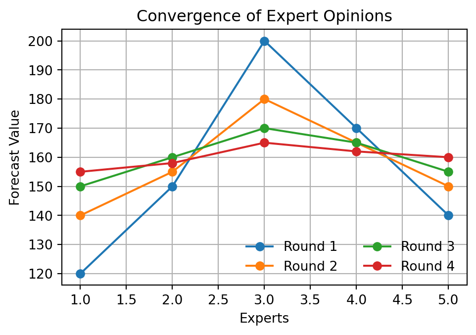
2 Quantitative Methods - Delphi Method
Delphi Method
A qualitative forecasting technique that uses a panel of experts who anonymously provide forecasts and opinions through multiple rounds of questionnaires.
Then, the reports are statistically aggregated and shared with the group after each round, allowing experts to revise their forecasts based on the feedback from others.
The process continues until a consensus is reached or a predefined number of rounds is completed.
The method is useful for forecasting in situations where there is a lack of historical data or when the future is highly uncertain, such as in new product development or technological forecasting.
Consensus is reached through multiple rounds of expert feedback.
The results indicate that
In the first round, experts give very different forecasts.
After seeing the summary of responses, they reconsider their estimates.
Over several rounds, opinions move closer together.
Once consensus is reached or the maximum number of rounds is completed, the final forecast can be used for decision-making in supply chain planning and operations.
3. Quantitative Methods
Quantitative forecasting methods use historical data and mathematical models to predict future values.
The examples include:
Naïve forecasting: Assumes the future will be the same as the most recent observation.
Regression analysis: Models the relationship between a dependent variable and one or more independent variables.
Moving average: Averages a fixed number of the most recent data points to smooth out fluctuations.
Exponential smoothing: Applies decreasing weights to past observations to forecast future values.
Time series decomposition: Breaks down a time series into trend, seasonal, and random components.
These methods are typically more objective and can be more accurate than qualitative methods when there is sufficient historical data available.
3.1 Pattern Analysis
Demand data often follows different patterns that influence the choice of forecasting method. The most common demand components are
Demand gradually increases or decreases over time.
Linear models, regression, Holt’s exponential smoothing
3.1 Pattern Analysis (cont.)
Seasonality
Regular and predictable fluctuations in demand that occur at specific intervals, such as weekly, monthly, or quarterly. Most commonly observed in retail.
In practice, demand data often contains a combination of these patterns, making forecasting more complex.
\[
\text{Demand = Trend + Seasonality + Random Variation}
\]
Pattern analysis is crucial for selecting the appropriate forecasting method and improving forecast accuracy.
The choice of forecasting method should be based on the dominant pattern in the data and the specific context of the supply chain problem being addressed.
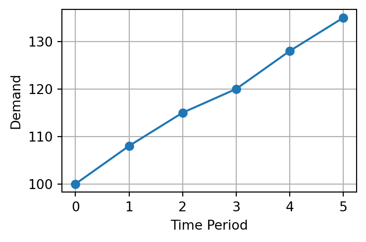
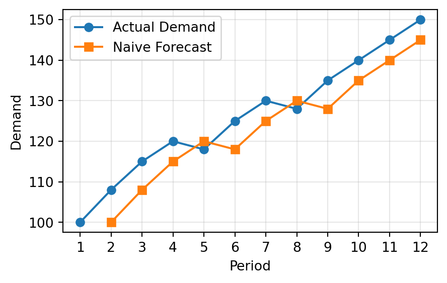
3.2 Naïve Forecasting
Assumes the next period forecast \(F_{t+1}\) will be the same as the current period,
\[
F_{t+1} = F_t
\]
Period
1
2
3
4
5
6
7
8
9
10
11
12
Demand \(F_t\)
100
108
115
120
118
125
130
128
135
140
145
150
Forecast \(F_{t+1}\)
-
100
108
115
120
118
125
130
128
135
140
145
Very simple to apply
Useful as a benchmark
Works better when demand is stable
Performs poorly when trend or seasonality exists
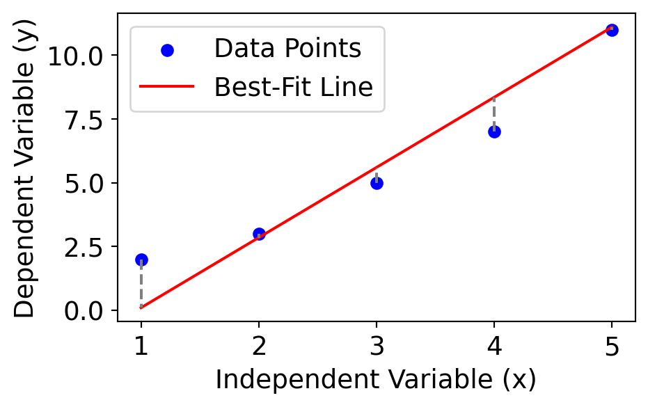
3.3 Regression Analysis
A statistical method for modelling the relationship between a dependent variable and one or more independent variables.
Commonly used to identify trends and make forecasts when data shows a linear pattern.
Equation of the Best-Fit Line
\[
\hat{y} = a + bx
\]
where \(\hat{y}\) is the predicted value, \(x\) is the independent variable, \(a\) is the intercept, and \(b\) is the slope of the line:
Figure 1. Forecasting of weekly sales based on TV promotional spend
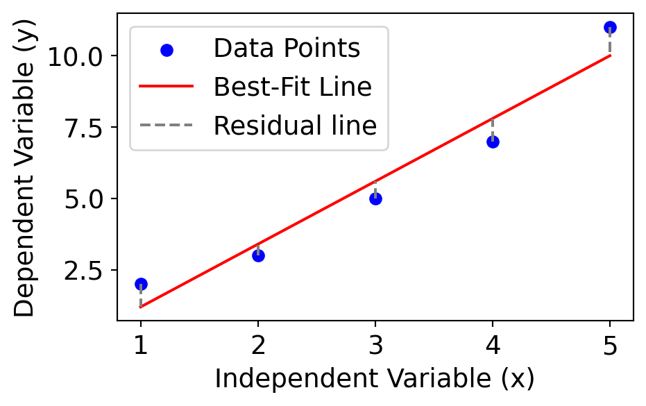
3.3.1 The Least Squares Method
In linear regression, the best-fit line is the straight line that most accurately represents the relationship between the independent variable (input) and the dependent variable (output). It is the line that minimises the residuals, given by: \[\text{Residual} = y_i - \hat{y}_i,\]
where \(y_i\) = the actual observed value and \(\hat{y}_i\) = predicted value
The least squares method minimises the sum of the squared residuals (SSE):
\[SSE = \sum (y_i - \hat{y}_i)^2\]
Figure 1. Forecasting of weekly sales based on TV promotional spend
3.3.2 Curve Fitting
Given \(n\) observations \((X_i, Y_i)\), we can fit a line to the overall pattern of these data points. From the Least Squares Method, we can calculate the slope \(b\) and intercept \(a\) using the following formula:
Slope (b) indicates how much the dependent variable (\(y\)) changes with each unit change in the independent variable (\(x\)). E.g. slope of 5 means that for every 1-unit increase in \(x\), the value of \(y\) increases by 5 units.
Intercept (a): The intercept represents the predicted value of \(y\) when \(x = 0.\) It is the point where the line crosses the y-axis.
3.3.3 Example
Predict the demand \(Y\) based on week number \(X\) using SLR.
The choice of number of periods will affect the forecasting results.
Smaller \(n\): more sensitive to changes (less smoothing)
Larger \(n\): more smoothing, but slower to react to shifts
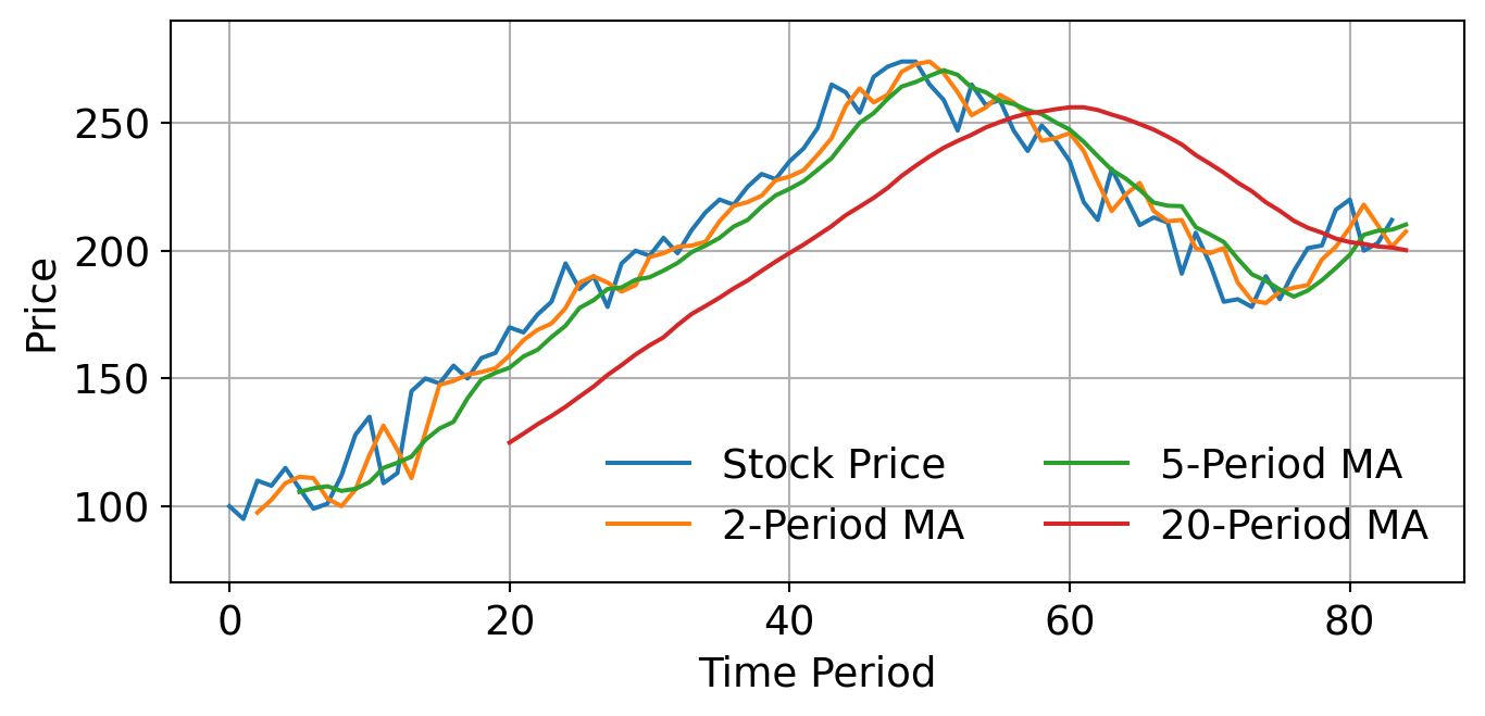
3.4.1 Moving Average in Finance
Moving averages are widely used in financial markets to analyse stock price trends and make trading decisions. They help investors identify potential buy or sell signals based on the relationship between short-term and long-term moving averages.
Figure 2. Stock Trading Using Moving Average
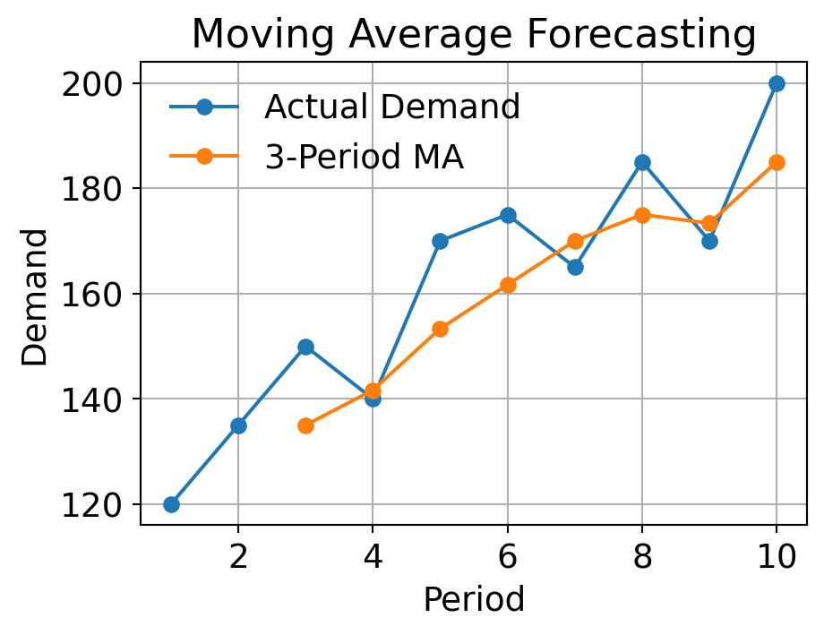
3.4.2 Example
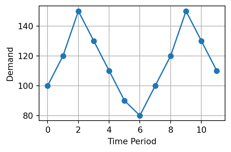
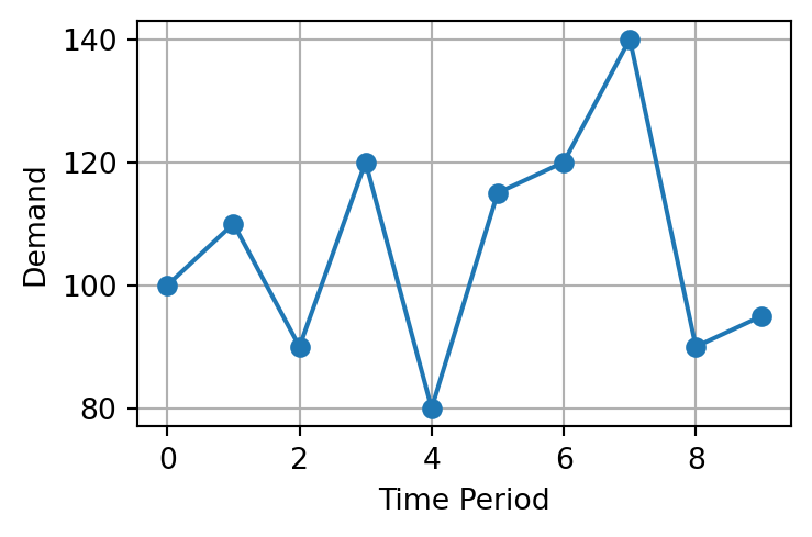
Given the historical demand from Period 1 to 10, use 3-period moving average to forecast the demand in Period 4 to Period 11.
Weights are all equal - all recent data treated the same (average)
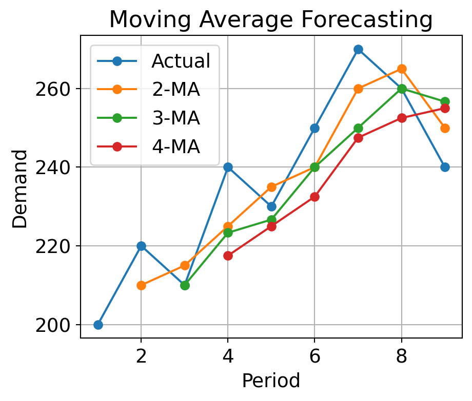
3.4.3 Exercise
A warehouse records the weekly demand (in units) for a specific component. Use moving averages with different periods to forecast demand and evaluate their effectiveness.
Week
1
2
3
4
5
6
7
8
9
Demand
200
220
210
240
230
250
270
260
240
Instructions:
Compute forecasts using:
2-period moving average
3-period moving average
4-period moving average
Start calculating forecasts only when you have enough prior data points.
Compute the SSE for each model.
Which moving average performed best?
How does increasing \(n\) affect the responsiveness of the model?
Which model would you choose if demand becomes more volatile?
3.4.3 Exercise (cont.)
1. Compute forecasts using 2-MA, 3-MA, and 4-MA
Period
Y
2-MA
3-MA
4-MA
1
200
2
220
3
210
4
240
5
230
6
250
7
270
240
8
260
260
250.00
9
240
265
260.00
252.50
10
250
256.67
255.00
3.4.3 Exercise (cont.)
2-3. Compute the SSE for each model. Which period MA performed best?
Period
Y
2-MA
3-MA
4-MA
1
200
2
220
3
210
4
240
5
230
6
250
7
270
240
8
260
260
250
9
240
265
260
252.50
3.5 Weighted Moving Average Model
A refinement of the simple moving average.
Assigns more importance (weight) to recent observations.
Better for data with slight trends, where recent periods are more relevant.
The choice of weights will affect the forecasting results.
Manual tuning: Try weights like (0.5, 0.3, 0.2) or (0.6, 0.3, 0.1)
Optimisation: Use historical error metrics to minimise forecast error
Heuristic: Emphasise recency, but balance for smoothing
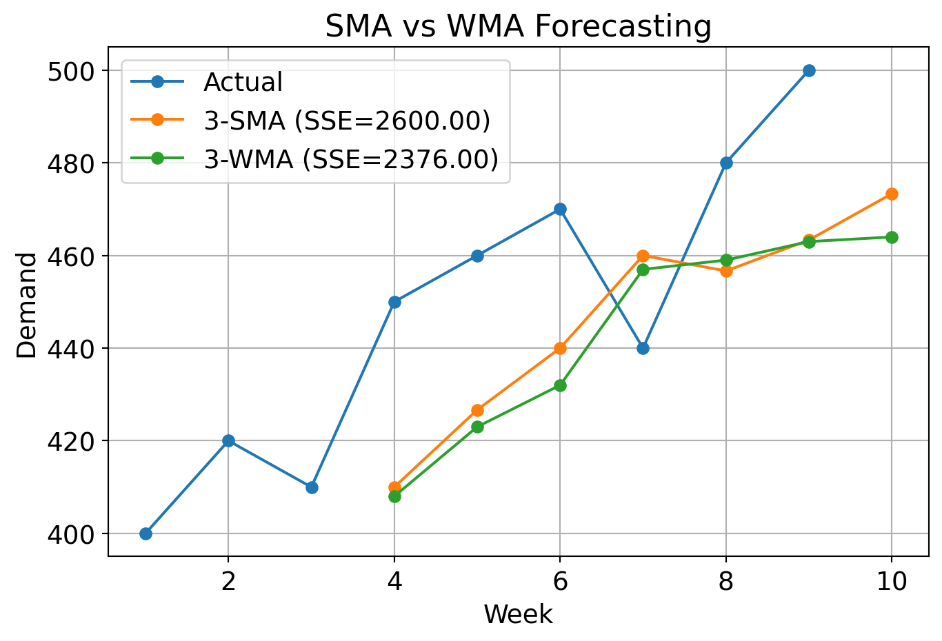
3.5.1 Example
A logistics manager tracks weekly outbound shipment volumes for a distribution center. To better anticipate outbound volume and optimize truck scheduling, you will forecast demand using both 3-period SMA and 3-period WMA with custom weights as follows:
Most recent: 0.5
Second recent: 0.3
Third recent: 0.2
Week
1
2
3
4
5
6
7
8
9
Demand
400
420
410
450
460
470
440
480
500
3.5.1 Example (cont.)
X
Y
3 MA
Error (SMA)
3 WMA
Error (WMA)
1
400
2
420
3
410
4
450
410.00
40.00
39
5
460
426.67
33.33
28
6
470
440.00
30.00
23
7
440
460.00
-20.00
-23
8
480
456.67
23.33
27
9
500
463.33
36.67
34
10
473.33
Which method performed better overall? Why?
3.5.1 Example (cont.)
Which method performed better overall? Why?
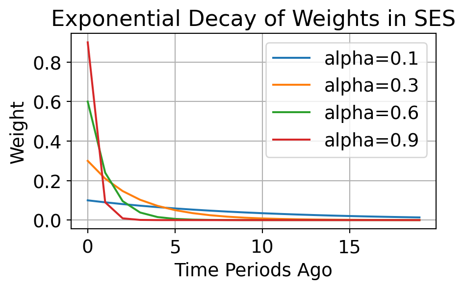
3.6 Simple Exponential Smoothing (SES)
SES generates forecasts by assigning exponentially decreasing weights to past observations.
Unlike moving averages, SES automatically adjusts the weight of new data through a smoothing parameter \(\alpha\).
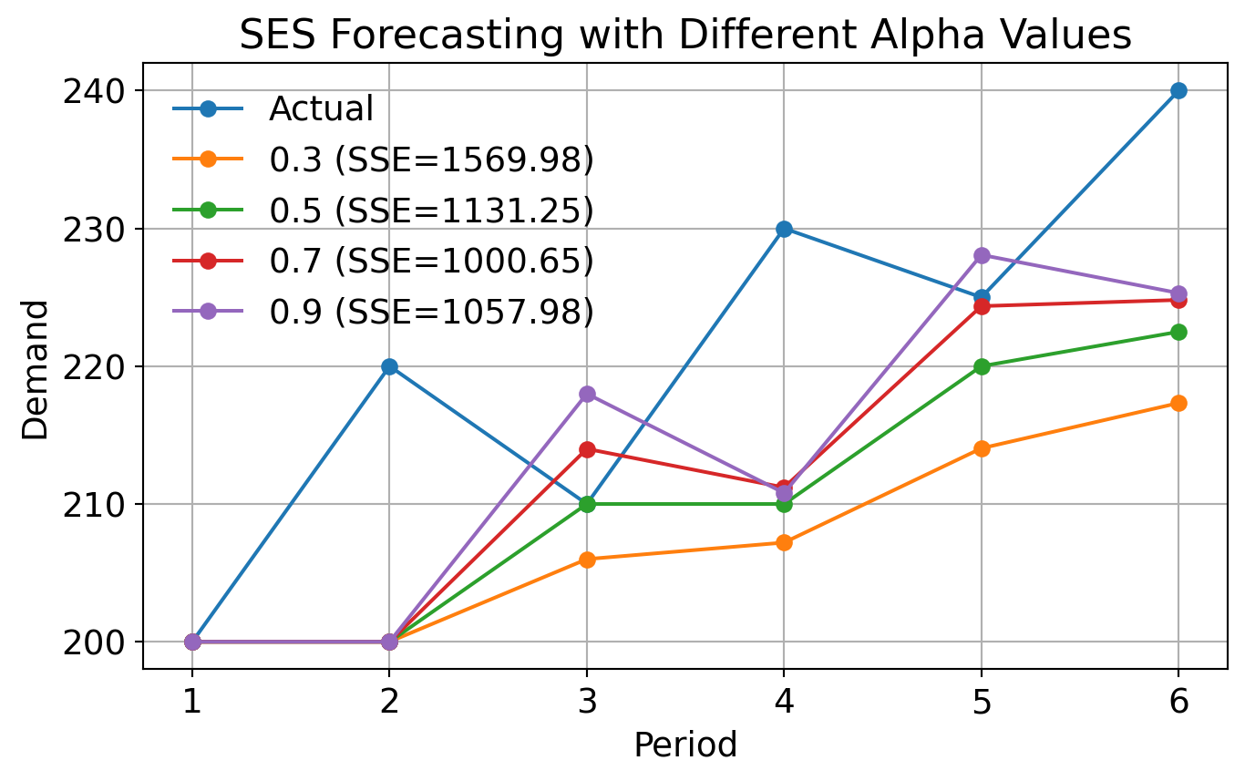
Conduct sensitivity analysis by varying \(\alpha\) and observing how the forecasts change. Try \(\alpha = [0.3, 0.5, 0.7, 0.9]\) and compare the results.
Code
import numpy as npactual = np.array([200, 220, 210, 230, 225, 240])alpha = [0.3, 0.5, 0.7, 0.9]forecasts = {}for a in alpha: forecast = np.empty_like(actual, dtype=float) forecast[0] =200# initial forecastfor t inrange(1, len(actual)): forecast[t] = a * actual[t-1] + (1- a) * forecast[t-1] forecasts[a] = forecast## sse for each alphasse = {a: np.sum((actual - forecasts[a]) **2) for a in alpha}plt.figure(figsize=(8, 4.5))plt.plot(np.arange(1, len(actual)+1), actual, marker='o', label='Actual')for a in alpha: plt.plot(np.arange(1, len(actual)+1), forecasts[a], marker='o', label=f'{a} (SSE={sse[a]:.2f})')plt.xlabel('Period')plt.ylabel('Demand')plt.title('SES Forecasting with Different Alpha Values')plt.legend(frameon=False)plt.grid()plt.show()
3.6.2 Example (cont.)
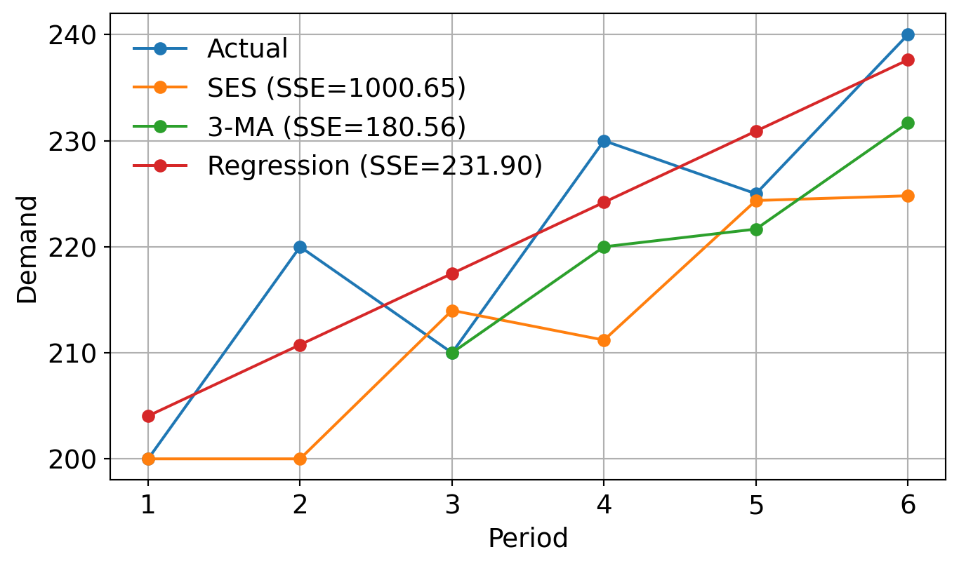
Calculate the SSE for the forecasts and discuss how well SES using the best \(\alpha\) performed compared to a simple moving average with a 3-period window and regression analysis.