Inventory: The stock of any item or resource used in an organisation.
Inventory system: Policies and controls to monitor stock levels and reorder timing/quantity.
Types of Inventory
Direct
Directly contributes to the production of finished goods. These are physical items that are integrated into the final product or play an active role in the manufacturing process.
Examples: Raw materials, WIP, finished goods, spare parts.
Indirect
Inventory that does not become part of the final product but is necessary to support the production or business operations.
Examples: Maintenance, Repair, and Operations (MRO) supplies, office supplies, tools, and equipment.
Inventory Metrics
Average aggregate inventory value
\[
\boxed{\sum_{\text{all items}}(\text{Avg Units} \times \text{Cost per Unit})}
\]
Weeks of Supply
\[
\boxed{\frac{\text{Avg aggregate inventory value}}{\text{the value of the sales per week}}}
\]
The total average value of inventory held across all items, which helps track the financial investment tied up in inventory.
How long the avg inventory can support demand.
High value: overstocking or slow-moving inventory.
Low value: lean inventory or potential stockouts.
The number of times inventory is sold and replaced in a year, indicating how efficiently inventory is being used.
High turnover: implies faster sales or better inventory control.
Low turnover: could signal overstocking, obsolete items, or slow sales.
1.2 Objectives of Inventory Management
An inventory model is a mathematical or analytical framework used by businesses to determine how much inventory to order, when to order it, and how to manage stock efficiently.
The main goal is to balance costs and service levels—ensuring that products are available when needed while minimising expenses associated with ordering and holding inventory.
Important
At its core, inventory management deals with three key questions:
How much to order?
When to order?
How to minimise total cost?
1.3 Inventory Cost Components
Inventory models help answer these questions by considering various cost components, such as
Component
Description
Purchase Cost (PC)
The amount paid to acquire inventory.
Inventory Holding Cost (IHC)
The cost of storing and maintaining inventory over time, including storage, insurance, depreciation, and capital.
Shortage Cost (SC)
The cost incurred when demand cannot be met due to stockouts, which includes lost sales and emergency orders.
Ordering Cost (OC)
The cost associated with placing an order or setting up a production batch.
Total Inventory Cost (TC)
With discount: \(TC = PC + IHC + SC + OC\); Without discount: \(TC = IHC + SC + OC\)
Objective: Determine the correct quantity to order that minimises the total cost.
1.4 Other Variables
Apart from costs, there are other variables which play an important role in decision-making,
Variable
Description
Planning Horizon
The period over which a particular inventory level will be maintained.
Demand
The quantity of inventory required to meet customer needs, which can be deterministic or probabilistic.
Lead-time
The time between placing an order and receiving it, which can be deterministic or probabilistic.
Cycle-time (T)
The time between placements of two orders.
Deterministic: The exact quantity and timing are predictable and do not vary over time.
Probabilistic: Uncertain and described using probability distributions.
1.5 Types of Inventory Models
More advanced models incorporate uncertainties in demand and lead time, such as probabilistic models, while others handle real-world complexities like bulk discounts or perishable goods.
Inventory models can be broadly classified into:
Deterministic models
assume demand and lead time are known and constant
Stochastic models
account for uncertainty and variability in demand or supply
Also, resupply strategies can be classified into:
Push System
Inventory is produced or ordered based on forecasted demand and pushed through the supply chain.
Pull System
Inventory is produced or ordered in response to actual demand, pulling products through the supply chain.
1.6 Multi-echelon Inventory Systems
%%{init: {
  "flowchart": {
    "htmlLabels": true,
    "padding": 5,
    "nodeSpacing": 35,
    "rankSpacing": 25
  },
  "theme": "base",
  "themeVariables": {
    "fontSize": "16px",
    "secondaryColor": "#ffffff"
  }
}}%%
flowchart LR

    %% ---------------------------
    %% Layer 1
    %% ---------------------------
    subgraph TOP[ ]
        direction LR
        MP([Manufacturing<br>Plant])
        FW([WHs])
    end

    %% ---------------------------
    %% Layer 2
    %% ---------------------------
    subgraph MID[ ]
        direction LR

        V([Vendors])
        RMI["RMI"]
        CPI["CPI"]
        WIP["WIP"]
        FGI["FGI"]
        W([W/S])
        R([RET])
    end

    %% ---------------------------
    %% Layer 3
    %% ---------------------------
    subgraph BOT[ ]
        direction LR
        DC([DCs])
    end

    %% Main flow
    V -->|Buying| RMI
    V -->|Buying| CPI
    RMI -->|Fabrication| CPI
    CPI -->|Initial<br>Assembly| WIP
    WIP -->|Final<br>Assembly| FGI

    FGI --> FW
    FGI --> DC
    FW --> W
    DC --> W
    W --> R

    %% Invisible alignment helpers
    MP --> RMI
    FW -.-> W
    RMI -.-> DC

    %% Styles
    classDef inventory fill:#ffffff,stroke:#d33,stroke-width:2px,stroke-dasharray: 6 4;
    classDef circle fill:#ffffff,stroke:#555,stroke-width:1.5px;
    classDef invisible fill:none,stroke:none,color:none;

    class RMI,CPI,WIP,FGI inventory;
    class V,FW,DC,W,R circle;
    class TOP,MID,BOT invisible;
    style MP fill:#ffffff,stroke:#ffffff;
Inventory is represented by red-dashed rectangles, while entities (e.g. vendors, warehouses) are represented by circles.
1.7 Analytical Tools for Inventory Management
EOQ and EPQ Models
Economic Order Quantity and Economic Production Quantity models are fundamental tools for determining optimal order quantities that minimise total inventory costs.
Optimisation Models
Optimisation models are used to determine the best order quantities and inventory policies that minimise costs or maximise service levels under various constraints.
Monte Carlo Simulation
A computational technique that uses random sampling to estimate the probability distribution of outcomes for complex inventory systems.
Newsvendor Model
The Newsvendor model is used to determine optimal order quantities for products with uncertain demand and a limited selling period.
2. Economic Order Quantity (EOQ) Model
For a single-stocking point, single-commodity inventory system with constant demand and lead time (deterministic), the parameters are as follows:
Notation
Unit
Description
\(C\)
$/unit
Purchase or manufacturing cost of an item
\(A\)
$/order
The ordering cost per order
\(h\)
$/unit/time
Inventory holding cost of an item per unit per time unit
\(k\)
$/unit/time
Shortage cost per unit short per time
\(D\)
units/time
Demand rate of per planning horizon, usually per year
\(S\)
units
Shortage quantity, a decision variable
\(Q\)
units
Order quantity, a decision variable
\(T\)
Time
Cycle time (time between orders), a decision variable
\(R\)
units
Reorder level (inventory level at which an order is placed)
\(L\)
Time
Lead time
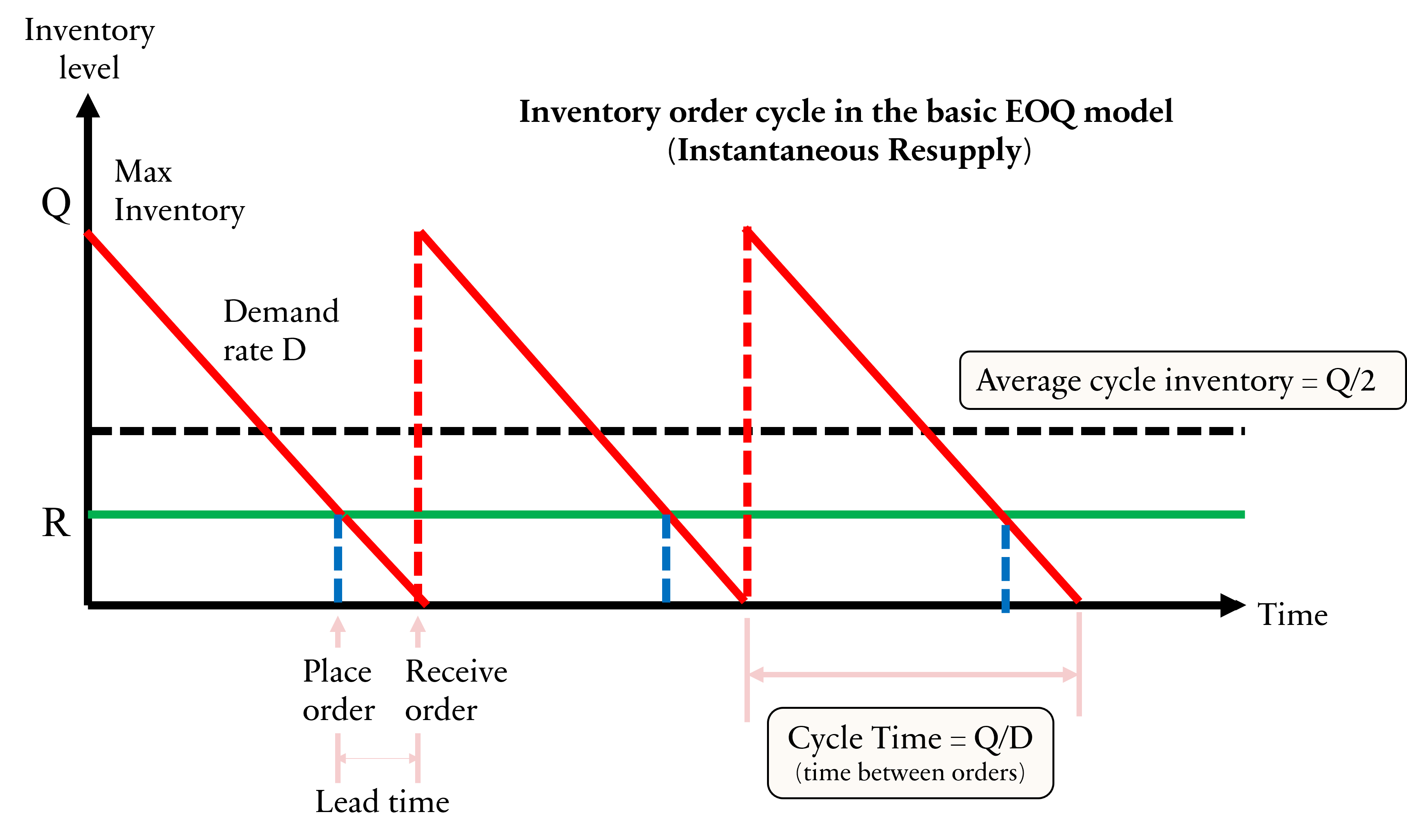
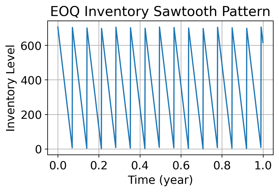
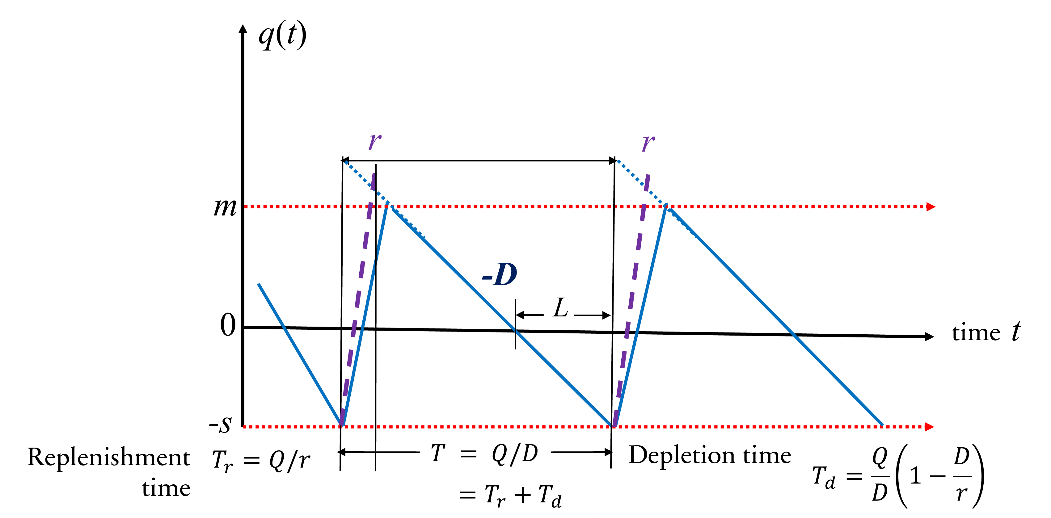
2.1 Inventory Order Cycle in the Basic EOQ Model
2.2 EOQ Model – Formula
Order Quantity
\[
\boxed{Q = D \times T}
\]
Demand rate multiplied by cycle time. Make sure that the units for demand rate and cycle time are consistent.
Ordering Cost
\[
\boxed{OC = \frac{D}{Q} \cdot A}
\]
\(D/Q\) is the number of orders placed during the planning horizon. \(A\) is the ordering cost per order.
Inventory Holding Cost
\[
\boxed{IHC = \frac{Q}{2} \cdot h}
\]
Average cycle inventory multiplied by holding cost per unit (\(h\)).
From the \(TC\) formula, determine the order quantity \(Q^*\) that minimises it.
Setting the first derivative of \(TC\) with respect to \(Q\) to zero and solving for \(Q\): \[
\frac{d}{dQ}TC = -\frac{D}{Q^2}A + \frac{h}{2} = 0 \implies \boxed{Q^* = \sqrt{\frac{2DA}{h}}},
\] where \(Q^*\) is the optimal order quantity or optimal lot size.
The minimum total cost is obtained by substituting \(Q^*\) back into \(TC\): \[
TC(Q^*) = \frac{D}{Q^*} \cdot A + \frac{Q^*}{2} \cdot h \implies \boxed{TC(Q^*) = \sqrt{2DAh}}
\]
If quantity discount is taken into account, then: \[
\boxed{TC = CD + \frac{D}{Q^*} \cdot A + \frac{Q^*}{2} \cdot h}
\]
How often should an order be placed to maintain inventory efficiently?
Cycle Time
\[
\boxed{T = \frac{Q^*}{D}}
\]
The time interval between placing two consecutive orders, in years, months, or days depending on units.
Number of orders placed per planning horizon, in years, months, or days depending on units.
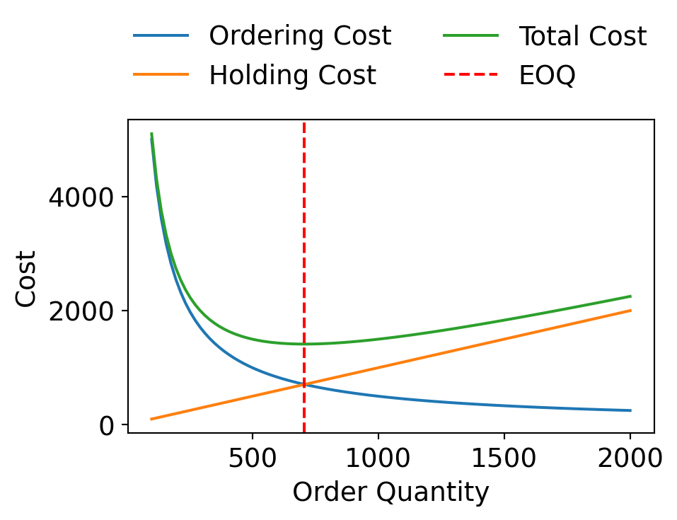
2.3 EOQ Cost Trade-Off
Let’s visualise the cost trade-off between ordering cost and holding cost, and how EOQ minimises total inventory cost. In this example, we will use the following parameters: \(D = 10000\), \(A = 50\), \(h = 2\).
At EOQ, Ordering Cost = Holding Cost
EOQ minimises total inventory cost
EOQ (Q*): 707.11 units
Cycle time (T): 0.0707 years
Large \(D\) → larger order quantity
High \(A\) → order less frequently (larger \(Q\))
High \(h\) → smaller order quantity
2.4 Sensitivity of the Lot-Size Model
Examines how changes in the order quantity from the optimal EOQ value affect the total cost.
It helps determine how critical it is to order exactly the EOQ, or whether near-optimal values are acceptable.
Why is it important?
We might not always order exactly EOQ due to supplier constraints, quantity discounts, or packaging sizes.
The total cost curve is relatively flat near EOQ, so minor deviations in order size result in minimal cost changes.
Example 3: A company uses rivets at a rate of 5,000 kg per year, with rivets costing $2 per kg. It costs $20 to place an order and the carrying cost of inventory is 10% per annum. How frequently should orders for rivets be placed and how much?
Example 4: A supplier ships 100 units of a product every Monday. The purchase cost of product is $60 per unit. The cost of ordering and transportation from the supplier is $150 per order. The cost of carrying inventory is estimated at 15% per year of the purchase cost. Find the lot-size that will minimise the cost of the system. Also determine the optimum inventory cost.
The total cost is only slightly higher when rounding up (almost no different).
So, the choice of rounding up or down does not significantly impact the total cost, and either option can be considered acceptable based on other factors such as storage space or risk tolerance.
Example 5. The annual demand for a certain item is 3,000 units per period. Unsatisfied demand causes a shortage cost of $0.75 per unit per year. The cost of initiating purchasing action is $15.00 per purchase and the holding cost is 15% of average inventory valuation per period. Item cost is $8.00 per unit. Find purchase quantity and the minimum inventory cost.
Example 6. A television manufacturing company produces its own speakers, which are used in the production of its television sets. The television sets are assembled on a continuous production line at a rate of 8,000 per month. The company is interested in determining when and how much to procure. Given.
Each time a batch is produced, a set-up cost of $12,000 is incurred.
The cost of keeping a speaker in stock is $0.30 per month.
The production cost of a single speaker is $10.00 and can be assumed to be a unit cost.
Shortage of a speaker, if it exists, costs $1.10 per month.
where \(A\) can also be interpreted as the setup cost per production run.
Setting the first derivative of \(TC\) with respect to \(Q^*\) to zero and solving for \(Q^*\):
Optimal lot size\[
\boxed{Q^* = \sqrt{\frac{2DA}{h}\frac{r}{r-D}}
= \sqrt{\frac{2DA}{h(1-D/r)}}}
\]
The term \(\frac{r}{r-D}\) accounts for the fact that production is not instantaneous but occurs gradually over time, which affects the average inventory level.
The minimum total cost is obtained by substituting \(Q^*\) back into \(TC\):
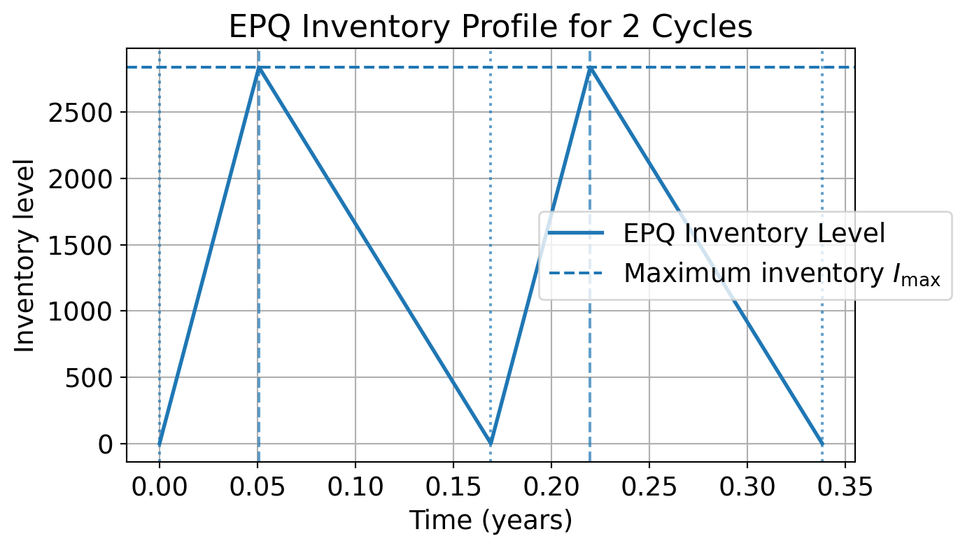
Example 9. A beverage company produces its own cardboard packaging boxes for shipping bottled drinks to retailers. The boxes are consumed continuously by the filling and packing line.
The following data are given:
Annual demand: \(D = 24{,}000\) boxes/year
Production rate: \(r = 80{,}000\) boxes/year
Demand rate: \(d = 24{,}000\) boxes/year
Setup cost per production run: \(A = \$120\)
Holding cost: \(h = \$0.50\) per box per year
Determine:
The optimal production lot size \(Q^*\)
The maximum inventory level
The total annual relevant cost
The optimal production lot size \(Q^*\) is calculated using the EPQ formula:
import numpy as npimport matplotlib.pyplot as plt# -----------------------------# EPQ parameters# -----------------------------D =24000# annual demandp =80000# production rate per yeard =24000# demand rate per yearK =120# setup costh =0.50# holding cost# -----------------------------# EPQ calculations# -----------------------------Q = np.sqrt((2* D * K) / (h * (1- d / p))) # optimal production lot sizetp = Q / p # production timeT = Q / d # cycle lengthImax = Q * (1- d / p) # maximum inventoryprint(f"EPQ lot size Q* = {Q:.2f}")print(f"Production time tp = {tp:.4f} years")print(f"Cycle length T = {T:.4f} years")print(f"Maximum inventory Imax = {Imax:.2f}")# -----------------------------# Build 2-cycle inventory curve# -----------------------------cycles =2points_per_segment =200time_vals = []inventory_vals = []for k inrange(cycles): cycle_start = k * T# Segment 1: production period (inventory rises at rate p-d) t_up = np.linspace(0, tp, points_per_segment) i_up = (p - d) * t_up# Segment 2: no-production period (inventory falls at rate d) t_down = np.linspace(tp, T, points_per_segment) i_down = Imax - d * (t_down - tp) time_vals.extend(cycle_start + t_up) inventory_vals.extend(i_up) time_vals.extend(cycle_start + t_down) inventory_vals.extend(i_down)time_vals = np.array(time_vals)inventory_vals = np.array(inventory_vals)# -----------------------------# Plot# -----------------------------plt.figure(figsize=(7, 4))plt.plot(time_vals, inventory_vals, linewidth=2, label="EPQ Inventory Level")plt.axhline(Imax, linestyle="--", label=r"Maximum inventory $I_{\max}$")# Mark cycle boundariesfor k inrange(cycles +1): plt.axvline(k * T, linestyle=":", alpha=0.7)# Mark production stop timesfor k inrange(cycles): plt.axvline(k * T + tp, linestyle="--", alpha=0.7)plt.xlabel("Time (years)")plt.ylabel("Inventory level")plt.title("EPQ Inventory Profile for 2 Cycles")plt.grid(True)plt.legend(loc="center right", bbox_to_anchor=(1.15, 0.5))plt.show()
EPQ lot size Q* = 4056.74
Production time tp = 0.0507 years
Cycle length T = 0.1690 years
Maximum inventory Imax = 2839.72
4. Reorder Point & Policy
When should we place an order to replenish inventory?
Order \(Q\) units when stock drops to reorder point \(R\).
Basic reorder level
\[
\boxed{R = D \times L}
\]
represents the amount of stock needed to cover demand during the lead time.
This is used when:
Lead time (\(L\)) is shorter than or equal to the cycle time \(T\).
There is only one order in progress at any time.
Adjusted Reorder Point
\[
\boxed{R = D \times L - n \times Q^*}
\]
\(n \times Q^*\) is demand that will be covered by previous orders already placed.
This is used when:
\(L > T\), i.e. multiple orders may be in flight during the lead time.
\(n\) is the number of orders that will arrive during the lead time, \(\lfloor L/T \rfloor\).
Example 9. Suppose we have a demand of 100 units/week and a lead time of 2 weeks. When should we place an order to replenish inventory assuming that the lead time is shorter than the cycle time?
\[
R = 100 \times 2 = 200 \text{ units}
\]
Place an order when stock falls to 200 units.
Example 10. Suppose we have a demand of 100 units/week, a lead time of 3 weeks, and an EOQ of 250 units. When should we place an order to replenish inventory?