Topic 7: Inventory Model: Discount and Multi-Commodity
05115130 Supply Chain Modelling and Optimisation
11 Jun 2026
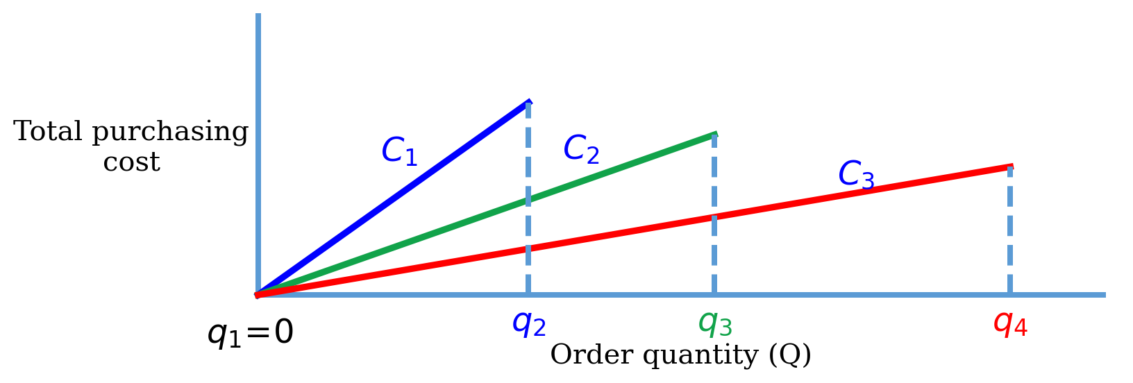
Quantity Discount Schedule (QDS)
| Discount Number | Discount Quantity | Discount | Discount Cost |
|---|---|---|---|
| 1 | 0 to 999 | 0% | $5.00 |
| 2 | 1000 to 1,999 | 4% | $4.80 |
| 3 | 2,000 and over | 5% | $4.75 |
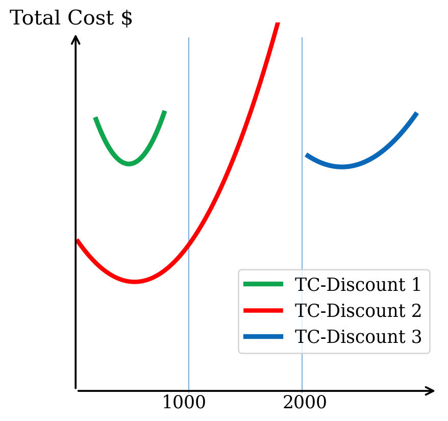
If \(Q^*\) for discount 2 in the QDS Table turns out to be 500 units (green TC), adjust this value up to 1,000 units to get 4% discount (red TC).
\[ \boxed{TC_i(Q) = C_𝑖 D +\frac{DA}{Q} + \frac{Q}{2} h_i}, \]
\[ \quad 𝑞_𝑖 \leq 𝑄 \leq 𝑞_{𝑖+1} \]
Code
import matplotlib.pyplot as plt

# Define key quantity breakpoints
q1, q2, q3, q4 = 0, 3, 6, 9

# Define piecewise cost curve (example values to match shape)
x = [0, q2, q3, q4]
y = [0, 8, 11, 12.5]  # increasing with decreasing slope

# Plot the main curve
plt.plot(x, y)

# Vertical dashed lines
plt.axvline(x=q2, linestyle='--', color='red')
plt.axvline(x=q3, linestyle='--', color='black')
plt.axvline(x=q4, linestyle='--')

# Labels for cost per unit regions
plt.text(q2/2, 4, "C₁/unit", ha='center', fontsize=14)
plt.text((q2+q3)/2, 9.5, "C₂/unit", ha='center', fontsize=14)
plt.text((q3+q4)/2, 12, "C₃/unit", ha='center', fontsize=14)

# Axis labels
plt.xlabel("Order Quantity (Q)", fontsize=14)
plt.ylabel("Total Purchasing Cost", fontsize=14)

# Ticks at q1, q2, q3, q4
plt.xticks([q1, q2, q3, q4], ['q1', 'q2', 'q3', 'q4'])

# Clean up appearance
plt.xlim(0, q4 + 1)
plt.ylim(0, max(y) + 2)

plt.show()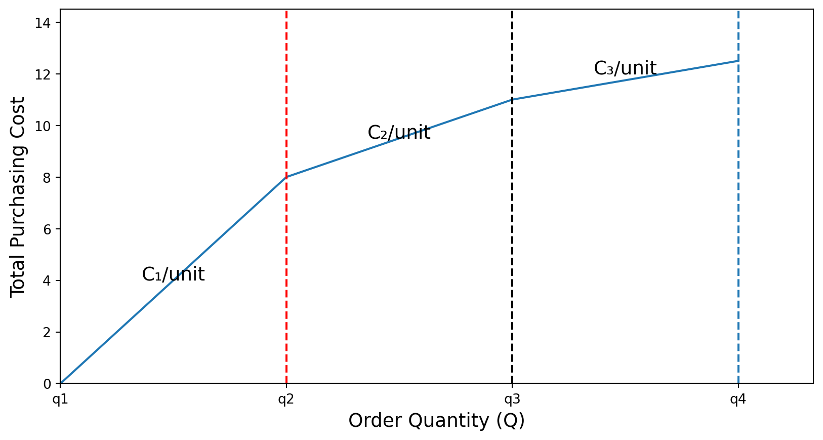
Code
import numpy as np
import matplotlib.pyplot as plt

# ----- Data -----
Q = np.linspace(0.12, 10, 800)

# Curves chosen to match the shape in the figure
y_red   = 2.8 / Q + 0.42 * Q + 0.1 #1.2
y_blue  = 1.3 / Q + 0.34 * Q + 0.9
y_green = 0.9 / Q + 0.55 * Q + 0.35
y_black = 0.45 / Q + 0.30 * Q + 1.25 #0.95

q1, q2, q3 = 0.8, 2.0, 5.6

# ----- Plot -----
fig, ax = plt.subplots(figsize=(8, 5.6))

ax.plot(Q, y_red,   'r--',  lw=2.8)
ax.plot(Q, y_blue,  'b-.',  lw=2.8)
ax.plot(Q, y_green, color='#00aa55', linestyle='-.', lw=2.8)
# ax.plot(Q, y_black, 'k-',   lw=3.0)

# Vertical dashed markers
ax.vlines(q1, ymin=0, ymax=np.interp(q1, Q, y_blue),  colors='k', linestyles='--', lw=1)
ax.vlines(q2, ymin=0, ymax=np.interp(q2, Q, y_black), colors='k', linestyles='--', lw=1)
ax.vlines(q3, ymin=0, ymax=np.interp(q3, Q, y_black), colors='k', linestyles='--', lw=1)

# Axes limits and labels
ax.set_xlim(0, 11)
ax.set_ylim(0, 12)
ax.set_xlabel('Order Quantity (Q)', fontsize=14, labelpad=12)
ax.set_ylabel('Total\nAnnual\nCost', fontsize=14, rotation=0, labelpad=42, va='center')

# Custom x-ticks
ax.set_xticks([q1, q2, q3])
ax.set_xticklabels(['q₁', 'q₂', 'q₃'], fontsize=14)

# Remove y-ticks to match the figure style
ax.set_yticks([])

# Style the frame
for spine in ax.spines.values():
    spine.set_linewidth(1.2)

ax.tick_params(axis='x', length=0, pad=8)
ax.tick_params(axis='y', length=0)

plt.tight_layout()
plt.show()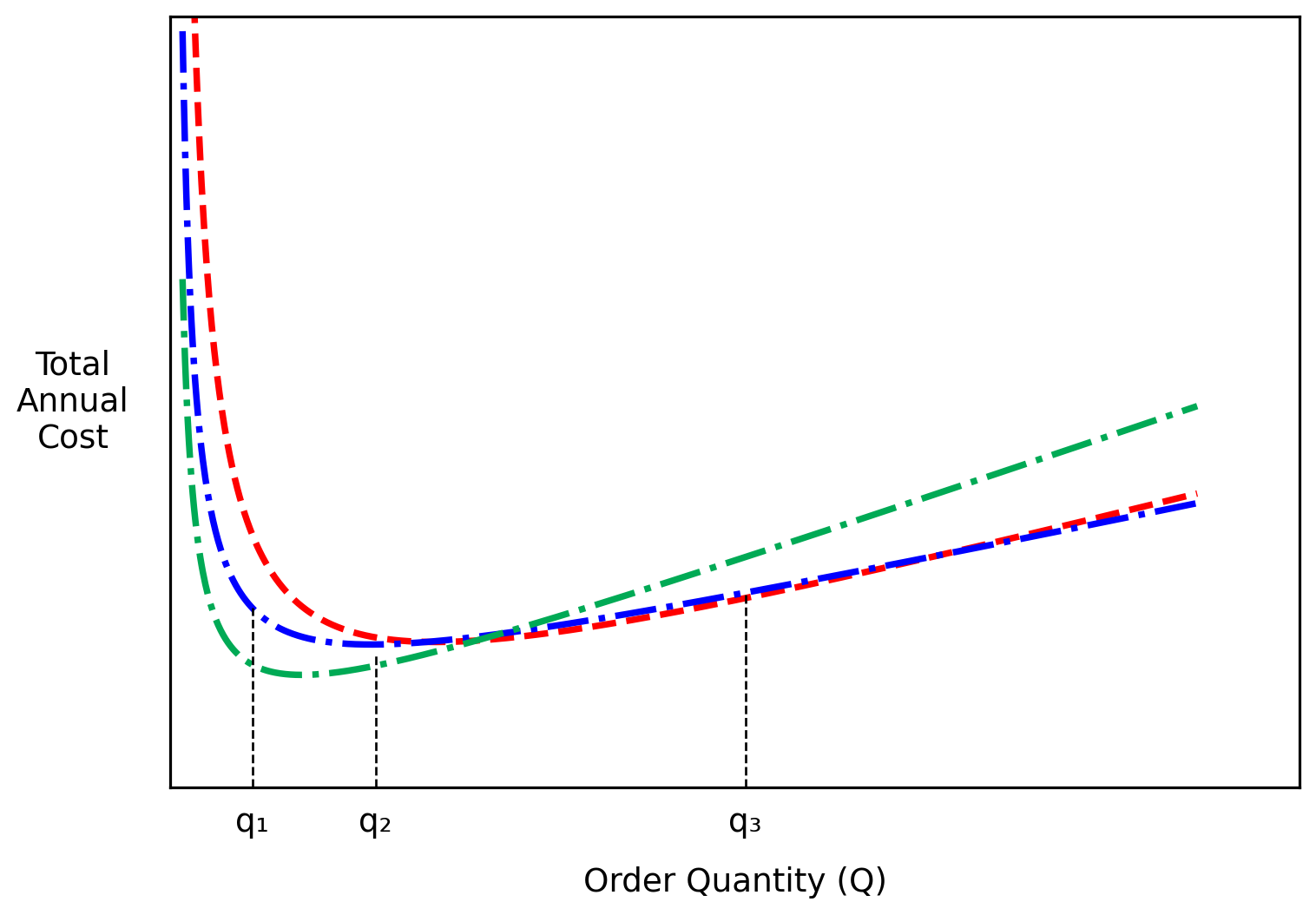
- A family of curves (dashed lines), each of which is valid for a given interval.
Code
import numpy as np
import matplotlib.pyplot as plt

# ----- Data -----
Q = np.linspace(0.12, 10, 800)

# Curves chosen to match the shape in the figure
y_red   = 2.8 / Q + 0.42 * Q + 0.1 #1.2
y_blue  = 1.3 / Q + 0.34 * Q + 0.9
y_green = 0.9 / Q + 0.55 * Q + 0.35
y_black = 0.45 / Q + 0.30 * Q + 1.25 #0.95

q1, q2, q3 = 0.8, 2.0, 5.6

# ----- Plot -----
fig, ax = plt.subplots(figsize=(8, 5.6))

ax.plot(Q, y_red,   'r--',  lw=2.8)
ax.plot(Q, y_blue,  'b-.',  lw=2.8)
ax.plot(Q, y_green, color='#00aa55', linestyle='-.', lw=2.8)
ax.plot(Q, y_black, 'k-',   lw=3.0)

# Vertical dashed markers
ax.vlines(q1, ymin=0, ymax=np.interp(q1, Q, y_blue),  colors='k', linestyles='--', lw=1)
ax.vlines(q2, ymin=0, ymax=np.interp(q2, Q, y_black), colors='k', linestyles='--', lw=1)
ax.vlines(q3, ymin=0, ymax=np.interp(q3, Q, y_black), colors='k', linestyles='--', lw=1)

# Axes limits and labels
ax.set_xlim(0, 11)
ax.set_ylim(0, 12)
ax.set_xlabel('Order Quantity (Q)', fontsize=14, labelpad=12)
ax.set_ylabel('Total\nAnnual\nCost', fontsize=14, rotation=0, labelpad=42, va='center')

# Custom x-ticks
ax.set_xticks([q1, q2, q3])
ax.set_xticklabels(['q₁', 'q₂', 'q₃'], fontsize=12)

# Remove y-ticks to match the figure style
ax.set_yticks([])

# Style the frame
for spine in ax.spines.values():
    spine.set_linewidth(1.2)

ax.tick_params(axis='x', length=0, pad=8)
ax.tick_params(axis='y', length=0)

plt.tight_layout()
plt.show()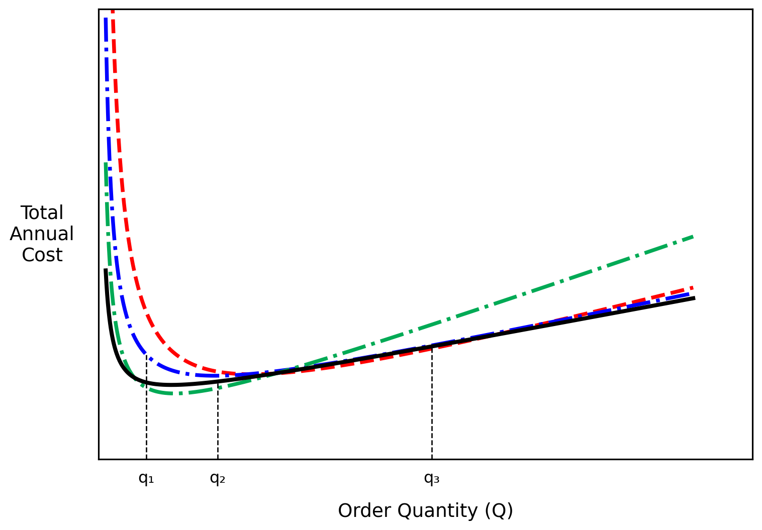
- A solid line (valid portion) constitutes the \(TC(Q)\) function.
Code
import matplotlib.pyplot as plt

# Figure
fig, ax = plt.subplots(figsize=(8, 5.5))

# Parameters
Q1 = 1.0
Q2 = 2.0
T1 = 1.2
T2 = 3 * T1   # big base = sum of 3 small bases

x0 = 0.7
x1 = x0 + T2

blue = "#5b93cf"
lw = 2.8

# -------------------------
# Big synchronized cycle
# -------------------------
ax.plot([x0, x0], [0, Q2], color=blue, lw=lw)          # jump up
ax.plot([x0, x1], [Q2, Q2], color=blue, lw=lw)         # top horizontal
ax.plot([x0, x1], [Q2, 0], color=blue, lw=lw)          # large decline

# second big cycle
ax.plot([x1, x1], [0, Q2], color=blue, lw=lw)
ax.plot([x1, x1 + T2], [Q2, 0], color=blue, lw=lw)

# -------------------------
# Small equal triangles
# -------------------------
small_starts = [x0 + i * T1 for i in range(6)]  # 3 in first big cycle, 3 in second

for s in small_starts:
    e = s + T1
    ax.plot([s, s], [0, Q1], color=blue, lw=lw)              # vertical jump
    ax.plot([s, e], [Q1, 0], color=blue, lw=lw)              # solid slope
    ax.plot([s + 0.10, e + 0.10], [Q1, 0],                   # dashed slope
            color=blue, lw=lw, ls=(0, (5, 4)))

# -------------------------
# Axis arrows
# -------------------------
ax.arrow(0, 0, 8.0, 0, length_includes_head=True,
         head_width=0.06, head_length=0.15, fc="black", ec="black", lw=2)
ax.arrow(0, 0, 0, 2.35, length_includes_head=True,
         head_width=0.12, head_length=0.08, fc="black", ec="black", lw=2)

# Tick marks and labels
ax.plot([-0.12, 0.25], [Q1, Q1], color="black", lw=1.3)
ax.plot([-0.12, 0.25], [Q2, Q2], color="black", lw=1.3)
ax.text(-0.22, Q1, r"$Q_1$", ha="right", va="center", fontsize=17)
ax.text(-0.22, Q2, r"$Q_2$", ha="right", va="center", fontsize=17)

# -------------------------
# T1 and T2 annotations
# -------------------------
y_t1 = 0.82
ax.annotate("", xy=(x0 + T1, y_t1), xytext=(x0, y_t1),
            arrowprops=dict(arrowstyle="->", color="gray", lw=1.8))
ax.text(x0 + T1/2, y_t1 + 0.08, r"$T_1$", ha="center", va="bottom", fontsize=18)

y_t2 = 2.08
ax.annotate("", xy=(x1, y_t2), xytext=(x0, y_t2),
            arrowprops=dict(arrowstyle="->", color="gray", lw=1.8))
ax.text((x0 + x1)/2, y_t2 + 0.02, r"$T_2 = 3T_1$", ha="center", va="bottom", fontsize=18)

# Axis label
ax.text(-0.05, 2.42, r"$q(t)$", ha="center", va="bottom", fontsize=18)

# Caption
fig.text(0.14, 0.03,
         "Fig 1. Inventory level as a function of time in the case of\nsynchronised order",
         fontsize=15, family="serif")

# Layout
ax.set_xlim(-0.35, 8.1)
ax.set_ylim(-0.15, 2.45)
ax.axis("off")

plt.show()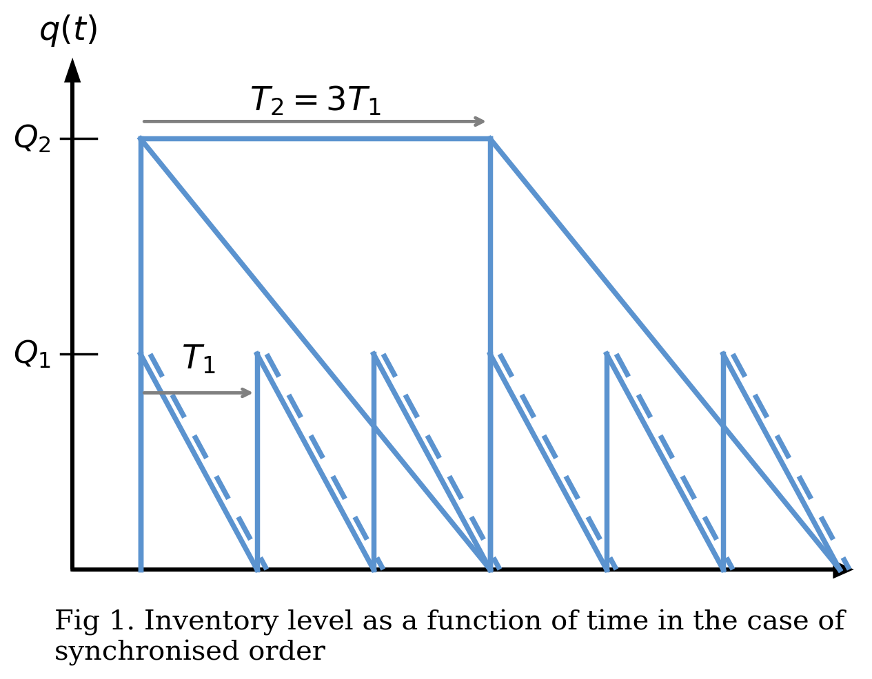
- Let \(T_1\) and \(T_2\) be the time lapses between consecutive replenishments of commodities 1 and 2, respectively.