Topic 8: Inventory Model: Inventory Control Policies and Stochastic Inventory Models

05115130 Supply Chain Modelling and Optimisation

Lecturer: Sam Wiwatanapataphee

275287a@curtin.edu.au

School of EECMS, Curtin University

12 Jun 2026

Outline

• 1. EOQ Reorder Point Review
  • 1.1 Basic EOQ and ROP
  • 1.2 Worked Example: Carpet Store
  • 1.3 Service-Level Intuition (bridge from stochastic models)
• 2. Continuous Review (Q, R) System
  • 2.1 Constant demand & constant lead time
  • 2.2 Variable demand & constant lead time
  • 2.3 Constant demand & variable lead time
  • 2.4 Variable demand & variable lead time

• 3. Periodic Review (P) System
  • 3.1 Basic mechanics and order-up-to level
  • 3.2 Worked Example: Bird Feeder Company
• 4. Choosing Between Q and P
  • 4.1 Comparison and decision rules
  • 4.2 Summary and key formulas
• 5. Single-Period Normal-Demand Model (Newsvendor)
  • 5.1 Critical ratio and optimal order quantity
  • 5.2 Expected cost under normal demand
  • 5.3 Worked example and interpretation

1. EOQ Reorder Point Review

Goal: Decide how much to order and when to order.

• EOQ gives order size; ROP gives order timing.

\[ \boxed{ROP = d \times L} \]

where \(d\) is demand rate and \(L\) is lead time.

Set the frame: quantity and timing are separate decisions. Remind students EOQ assumes steady demand and known costs. Emphasize units consistency for d and L. Students often mix annual and daily units in one formula. Transition to the EOQ and ROP formulas on the next slide.

Plot: EOQ Inventory Model with Reorder Point Across Multiple Cycles Demand: The inventory level decreases linearly at the rate D from EOQ to zero over the cycle time, with reorder points marked at ROP level. Each time inventory hits ROP, an order is placed, and inventory resets to EOQ after lead time. Lead time: time between order placed and the delivery.

We reserve capital \(D\) for annual demand and lowercase \(d\) for demand rate in consistent time units.

1.1 Basic EOQ and ROP

For annual demand \(D\), ordering cost \(K\), and annual holding cost \(h\):

\[ \boxed{Q^* = \sqrt{\frac{2KD}{h}}} \]

• \(Q^*\) optimal batch size to minimise total cost.
• EOQ does not include safety stock; it is the ideal order quantity under deterministic assumptions.

Then,

\[ ROP = d \times L \]

• \(ROP\) protects demand during replenishment lead time.

What happens if lead time doubles?

Walk through each symbol before substituting numbers. Highlight that EOQ does not include safety stock by itself. Use plain language: Q star is batch size, ROP is trigger level. Ask a quick check question about what happens if lead time doubles. Ans: ROP doubles, so you need to reorder sooner to avoid stockouts. Transition to the carpet-store worked example.

We sometimes use \(A\) and \(K\) interchangeably for ordering cost, but here we stick to \(K\).

1.2 Worked Example: Carpet Store

The carpet store wants to determine the optimal order size and total inventory cost given an estimated demand of 10,000 yards of carpet, an annual carrying cost of $0.75 per yard, and an ordering cost of $150. The store would also like to know the number of orders that will be made annually and the time between orders (i.e., the order cycle) given that the store is open 311 days per year. The lead time to receive an order is 10 days, determine the reorder point for carpet.

Given:

• \(D = 10{,}000\) yards/year
• \(K = 150\) dollars/order
• \(h = 0.75\) dollars/yard/year

• Store open 311 days/year
• Lead time \(L = 10\) days

Compute EOQ:

\[ Q^* = \sqrt{\frac{2(150)(10000)}{0.75}} \approx 2000\ \text{yards} \]

• Orders per year:

\[ n = \frac{D}{Q^*} = \frac{10000}{2000} = 5 \]

• Order cycle length:

\[ T = \frac{311}{5} \approx 62.2\ \text{days} \]

• Demand rate per day and reorder point:

\[ d = \frac{10000}{311} \approx 32.15, \quad ROP = dL \approx 32.15(10) \approx 322\ \text{yards} \]

Do the first substitution slowly so students see calculator steps. Remind class this example is deterministic in the first pass. Keep arithmetic visible and pause after EOQ result. Prompt students to estimate whether 2000 seems large or small. Transition: now compute cycle length and reorder point.

Reinforce that ROP is based on lead-time demand only. Clarify that cycle length and lead time are different concepts. Use the rounded value 322 for policy communication. Mention practical rounding to pack or pallet sizes if needed. Transition: add uncertainty with a short service-level bridge.

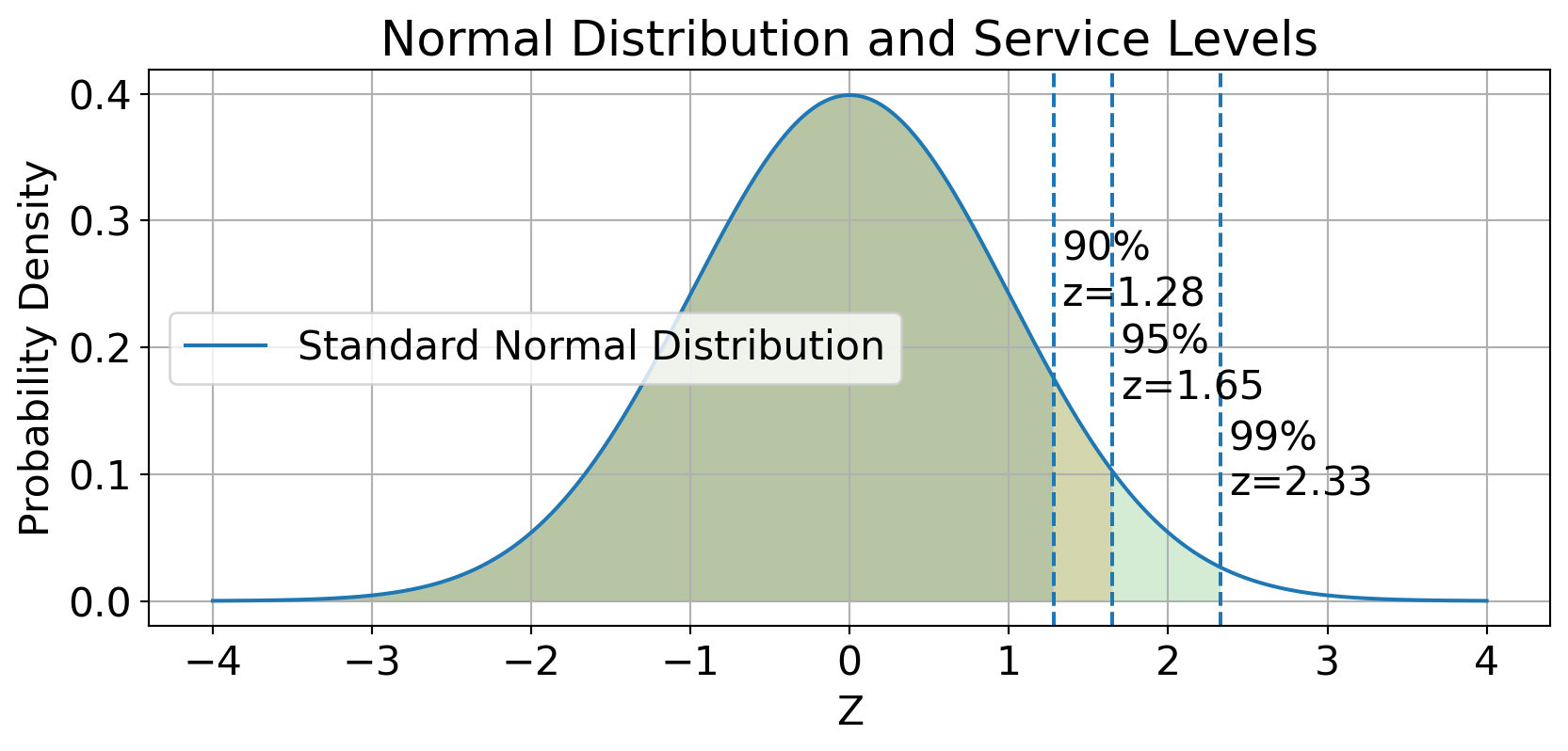
1.3 Service-Level Intuition (Bridge)

When demand is uncertain, use safety stock:

\[ \boxed{ROP = \bar{d}L + SS}, \quad \boxed{SS = z\sigma_L} \]

• \(z\) corresponds to target cycle-service level.
• Typical values: 90% (\(z \approx 1.28\)), 95% (\(z \approx 1.645\)), 99% (\(z \approx 2.33\)).
• Higher service level means more safety stock and higher holding cost.

This is the only bridge from stochastic lecture content we keep. Explain z as policy choice, not a random number to memorize. State the trade-off clearly: service versus inventory cost. Transition into continuous review where this formula is central.

Safety stock (SS) is the extra inventory you keep on hand as a buffer to protect against uncertainties.

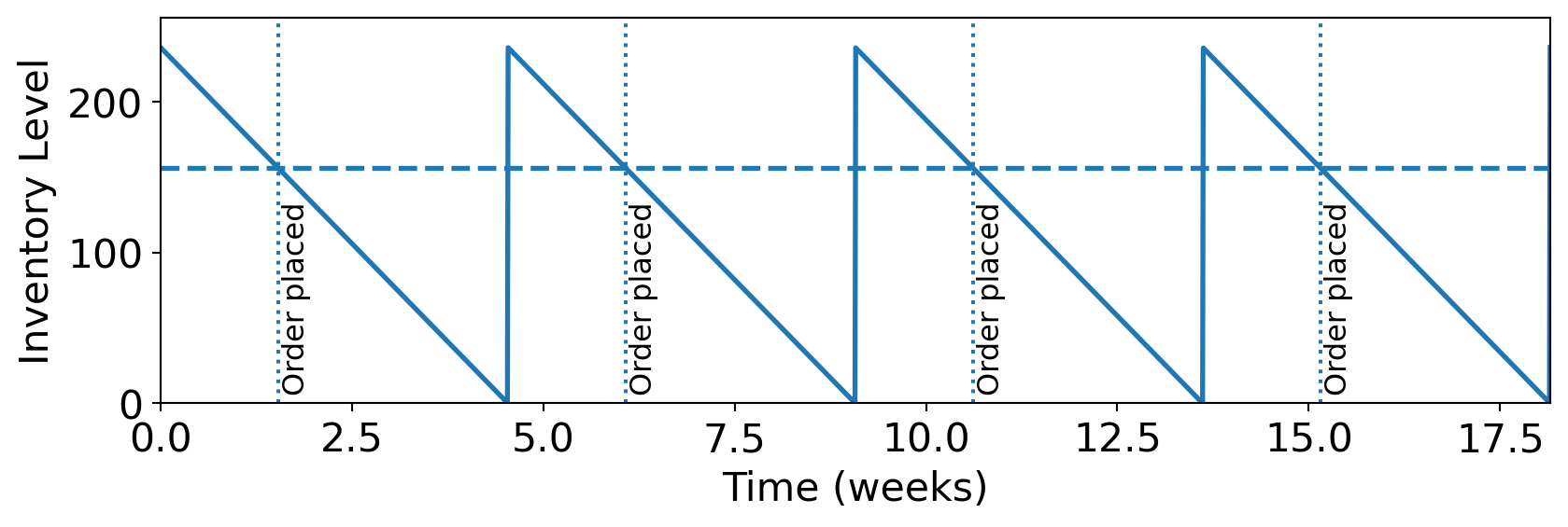
2. Continuous Review (Q, R) System

• Inventory position is monitored continuously.
• Place an order of fixed size \(Q\) when inventory reaches \(R\).
• Main strengths:
  • responsive to demand changes,
  • lower average inventory for similar service levels.

We will cover four cases:

Constant demand & constant lead time

Variable demand & constant lead time

Constant demand & variable lead time

Variable demand & variable lead time

Define inventory position briefly: on-hand plus on-order minus backorders. Stress that order quantity is fixed in Q-system. Students may confuse on-hand with inventory position; clarify now. Use a quick real-world example such as high-value spare parts, where continuous monitoring is feasible and desirable. Transition to the simplest deterministic case first.

2.1 Constant Demand and Constant Lead Time

If demand and lead time are both stable:

\[ \boxed{R = dL} \]

Example: \(d = 100\) units/week and\(L = 2\) weeks

\[ R = 100(2) = 200\ \text{units} \]

• Interpretation: place order whenever inventory position hits 200.

This works as the deterministic baseline policy.

Keep this slide fast to build confidence before uncertainty cases. Point out this is the deterministic baseline policy. Ask students what changes if demand rises to 120 units/week. Confirm they can recompute R in one line. Transition to uncertain demand and safety stock.

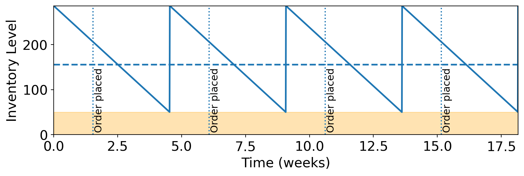
2.2 Variable Demand and Constant Lead Time

With uncertain demand and fixed lead time:

\[ \boxed{ROP = \bar{d}L + SS} \]

\[ \boxed{SS = z\sigma_L}, \quad \boxed{\sigma_L = \sigma_d\sqrt{L}} \]

where:

• \(\bar{d}\) is average demand rate during lead time.
• \(\sigma_d\) is standard deviation of demand per time unit.
• \(\bar{d}L\) covers expected lead-time demand.
• \(SS\) buffers demand variability during lead time.
• \(z\) corresponds to the desired service level.

Explain why square root of L appears in sigma L. Because demand variance accumulates over time, and standard deviation grows with the square root of time.

Tie z to target probability of no stockout during one cycle. Mention this formula is one of the most used in practice. Transition to a short numerical milk-inventory example.

• \(z\) corresponds to the desired service level.
  • Higher \(z\) means more safety stock and higher service level.
  • The value of \(z\) can be found from standard normal distribution tables based on the target service level (e.g., 1.28 for 90%, 1.645 for 95%, 2.33 for 99%).

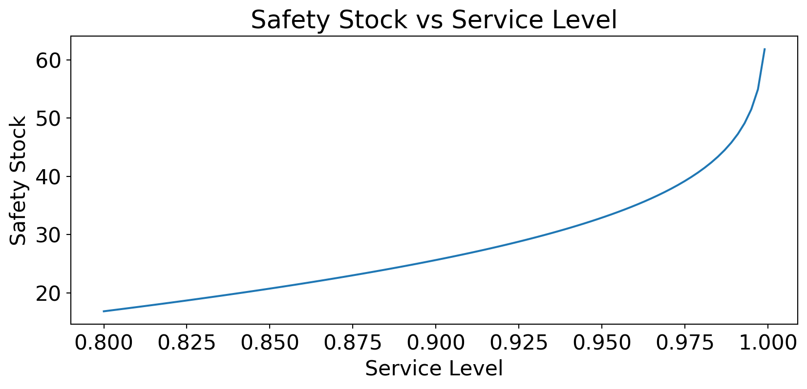
• The relationship between service level and safety stock is nonlinear.
  • As service level approaches 100%, the required safety stock increases dramatically.
  • This is because the tail of the normal distribution becomes thinner, requiring more inventory to cover rare demand spikes.

2.2 Worked Example: Bird Feeders

Suppose that the average demand for bird feeders is 18 units per week with a standard deviation of 5 units. The lead time is constant at 2 weeks. Determine the safety stock and reorder point for a 90 percent cycle-service level.

• \(\bar{d} = 18\) units/week
• \(\sigma_d = 5\) units/week

• \(L = 2\) weeks
• Service level = 90%, so \(z = 1.28\)

Compute lead-time demand deviation:

\[ \sigma_L = 5\sqrt{2} \approx 7.07 \]

Safety stock at 90% service level:

\[ SS = 1.28(7.07) \approx 9 \text{units} \]

Reorder point:

\[ ROP = \bar{d}L + SS = 18(2) + 9 \approx 45 \text{units} \]

2.2 Worked Example: Supermarket Milk Inventory

A supermarket sells milk and wants to avoid running out while waiting for new deliveries. Given

• Average demand = 200 cartons per week
• Delivery lead time = 3 weeks
• Demand variability = ±20 cartons/week
• Desired service level = 95% (very low chance of stockout)

Determine safety stock and reorder point.

From the problem statement:

• \(\bar{d} = 200\) cartons/week
• \(\sigma_d = 20\) cartons/week
• \(L = 3\) weeks
• Service level = 95%, so \(z = 1.645\)

Compute lead-time demand deviation:

\[ \sigma_L = 20\sqrt{3} \approx 34.64 \]

Safety stock at 95% service level:

\[ SS = 1.645(34.64) \approx 57 \]

Reorder point:

\[ ROP = \bar{d}L + SS = 200(3) + 57 = 657\ \text{cartons} \]

Policy statement:

• Monitor continuously.
• Place fixed order quantity \(Q\) when inventory position reaches 657.

What happens to SS if service target goes to 99%?

Ans: z increases to 2.33, so SS would be 2.33x34.64 ≈ 80.7 cartons, and ROP would increase to 200x3 + 80.7 ≈ 680.7 cartons.

2.3 Constant Demand and Variable Lead Time

If demand is stable but lead time varies:

\[ \boxed{R = d\bar{L} + SS}, \quad \boxed{SS = zd\sigma_{LT}} \] where:

• \(\bar{L}\) is average lead time.
• \(\sigma_{LT}\) is standard deviation of lead time.

Example: A store sells about 10 digital cameras a day. Lead time For camera delivery is normally distributed with a mean time of 6 days and a standard deviation of 3 days. A 95% service level is set. Find the reorder point.

• \(d = 10\) units/day
• \(\bar{L} = 6\) days

• \(\sigma_{LT} = 3\) days
• 95% service so \(z = 1.645\)

\[ R = 10(6) + 1.645(10)(3) = 109.35 \approx 109 \]

Compare this directly with previous case to show symmetry. Only uncertainty source changed from demand to lead time. Highlight unit checks: sigma LT in days, d in units per day. Students often forget to multiply z by d and sigma LT. Transition to the full variable-demand and variable-lead-time case.

2.4 Variable Demand and Variable Lead Time

When both demand and lead time are variable:

\[ \boxed{ROP = \bar{d}\bar{L} + SS}, \qquad \boxed{SS = z\sqrt{\bar{L}\sigma_d^2 + \bar{d}^2\sigma_L^2}} \]

• Sometimes written as \(SS = z\sigma_{dL}\) where \(\sigma_{dL}\) is the combined standard deviation of demand during lead time.

Example: A store’s most popular item is 9-volt battery. About 150 batteries are sold per day, following a normal distribution with a standard deviation of 16 batteries. Batteries are ordered from an out-of-state distributor; lead time is normally distributed with an average of 5 days a standard deviation of 1 day. To maintain a 95% service level, what ROP is appropriate?

• \(\bar{d}=150\), \(\sigma_d=16\) (units/day)
• \(\bar{L}=5\), \(\sigma_L=1\) (days)
• 95% service, \(z=1.645\)

Compute combined deviation:

\[ \sigma_{dL} = \sqrt{5(16)^2 + (150)^2(1)^2} \approx 154 \]

Safety stock:

\[ SS = 1.645(154) \approx 253 \]

Reorder point:

\[ ROP = 150(5) + 253 \approx 1003\ \text{units} \]

Keep arithmetic segmented into three short lines. Emphasize interpretation: large sigma L term can dominate quickly. Use this as a checkpoint before moving to P-system. Ask one conceptual question: why is P-system usually carrying more SS? Transition: now switch from continuous monitoring to periodic review.

Exercise: Grey Wolf Lodge is a popular 500-room hotel in the North Woods. Managers need to keep close tabs on all room service items, including a special pine-scented bar soap. The daily demand for the soap is 275 bars, with a standard deviation of 30 bars. Ordering cost is $10 and the inventory holding cost is $0.30/bar/year. The lead time from the supplier is 5 days, with a standard deviation of 1 day. The lodge is open 365 days a year.

1. What is the economic order quantity for the bar of soap?
2. What should the reorder point be for the bar of soap if management wants to have a 99 percent cycle-service level?
3. What is the total annual cost for the bar of soap, assuming a Q system will be used?

• Given:
  • \(D=275 \times 365\), \(K=10\), \(h=0.30\),
  • \(\bar{d}=275\), \(\sigma_d=30\), \(\bar{L}=5\), \(\sigma_L=1\),
  • service level = 99% so \(z=2.33\).

1. EOQ \[ Q^* = \sqrt{\frac{2KD}{h}} = \sqrt{\frac{2(10)(275 \times 365)}{0.30}} \approx 2,587\ \text{bars} \]

2. Reorder point: \[ \begin{aligned} ROP &= \bar{d}\bar{L} + z\sqrt{\bar{L}\sigma_d^2 + \bar{d}^2\sigma_L^2} \\ &= 275(5) + 2.33\sqrt{5(30)^2 + (275)^2(1)^2} \\ &\approx 2,035\ \text{bars} \end{aligned} \]

3. Total annual cost: \[ \begin{aligned} TC &= \frac{D}{Q^*}K + \left(\frac{Q^*}{2} + SS\right)h \\ &= 388 + 586 \\ &\approx \$974.06 \end{aligned} \]

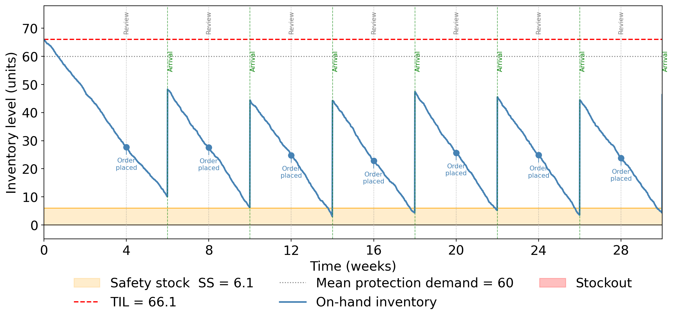
3. Periodic Review (P) System

Feature	Description
Review Interval \((P)\)	Orders are placed every \(P\) periods (e.g., every 4 weeks).
Order Quantity \((Q)\)	Varies each cycle; depends on how much is needed to “top up” to a target inventory level.
Target Inventory Level \((TIL)\)	A pre-set level that the inventory should reach after each order.
Lead Time \((L)\)	Time taken for the order to arrive after it’s placed.
Safety Stock \((SS)\)	Extra stock to cover demand variability during the protection period = \((P + L)\).

Core idea

\[ \text{Order quantity} = TIL - \text{inventory position at review} \]

Reinforce key contrast: fixed review schedule, variable order quantity. Define protection period verbally as P plus L. Students may think P-system has fixed order size; correct that. Give practical context: weekly ordering calendars with suppliers. Transition to deterministic TIL formula first.

Simulating a Periodic Review (P) System with Uncertain Demand and Lead Time with d = 10 units/week, σ_d = 0.8 units/week, P = 4 weeks, L = 2 weeks, and a 99.9% service level (z ≈ 3.09). The plot shows inventory levels over time, with safety stock shaded and markers for reviews, orders, and arrivals.

3.1 Basic Mechanics and Order-Up-To Level

For a Periodic Review System with review period \((P)\), average demand \((\bar d)\), average lead time \((\bar L)\), demand standard deviation per unit time \((\sigma_d)\), lead-time standard deviation \((\sigma_L)\), and service factor \((z)\):

Case	Safety Stock (SS)	Order-Up-To Level (TIL)
No uncertainty	\(0\)	\(\boxed{TIL=d(P+L)}\)
Demand uncertainty	\(\boxed{SS=z\sigma_d\sqrt{P+L}}\)	\(\boxed{TIL=\bar d(P+L)+z\sigma_d\sqrt{P+L}}\)
Lead time uncertainty	\(\boxed{SS=zd\sigma_L}\)	\(\boxed{TIL=d(P+\bar L)+zd\sigma_L}\)
Demand + lead time uncertainty	\(\boxed{SS=z\sqrt{\sigma_d^2(P+\bar L)+\bar d^2\sigma_L^2}}\)	\(\boxed{TIL=\bar d(P+\bar L)+z\sqrt{\sigma_d^2(P+\bar L)+\bar d^2\sigma_L^2}}\)

If using the EOQ-based optimal review period \(\boxed{T=\frac{Q^*}{\bar d}=\sqrt{\frac{2K}{\bar d h}}}\)

then simply replace \(P\) with \(T\): \(\boxed{I_{\max}=TIL}\)

Case	Maximum Inventory Level \(I_{\max}\)
No uncertainty	\(\boxed{\bar d(T+\bar L)}\)
Demand uncertainty only	\(\boxed{\bar d(T+\bar L)+z\sigma_d\sqrt{T+\bar L}}\)
Lead time uncertainty only	\(\boxed{\bar d(T+\bar L)+z\bar d\sigma_L}\)
Demand + lead time uncertainty	\(\boxed{\bar d(T+\bar L)+z\sqrt{\sigma_d^2(T+\bar L)+\bar d^2\sigma_L^2}}\)

\[ \text{TIL}=\text{Expected demand during protection period}+\text{Safety stock} \]

where the protection period is \(\boxed{P+\bar L}\).

(or \(T+\bar L\) when using the EOQ-derived review period).

3.2 Worked Example: Bird Feeder Company

A bird feeder company uses a periodic review (\(P\)) inventory system. Weekly demand is normally distributed with an average of 30 units and a standard deviation of 10 units. The supplier lead time is 2 weeks, and the company operates year-round (52 weeks annually). The system specifies an EOQ of 75 units and maintains safety stock to achieve a 95% cycle-service level. Determine the review period \(P\) and the targeted inventory level \(TIL\) for this system.

• Review period \(P\)
  • Given EOQ = 75 units, average period demand \(\bar{d}=30\;\) units
  • \(\displaystyle P = \frac{EOQ}{\bar{d}} = \frac{75}{30} = 2.5\;\) weeks
• Targeted inventory level \(TIL\)
  • \(SS = z \sigma_d \sqrt{P+L} = (1.645)(10)(\sqrt{2.5+2}) =34.8957\quad\) units
  • \(TIL= \bar{d} \times (P+L) + SS = (30)(2.5+2) + 34.8957=169.8957\quad\) units

4. Choosing Between Q and P

• Both systems use service level and safety stock ideas.
• Main design difference is review cadence and order quantity behavior.
• Selection should reflect data quality, IT capability, and operational rhythm.

Feature	Continuous (Q, R)	Periodic (P)
Review frequency	Continuous	Every \(P\) time units
Order size	Fixed (\(Q\))	Variable
Reorder trigger	Inventory position reaches \(R\)	Scheduled review
Typical safety stock	Lower	Higher
Monitoring effort	Higher	Lower

Decision rules

• Use Q-system for high-value or critical items.
• Use P-system when orders are synchronised on fixed schedules.
• Takeaway: EOQ sets size, ROP/TIL set timing and protection.

Move from formulas to managerial decision-making. Tell students exam and practice both require policy justification. Encourage thinking in context, not formula memorization only. Set up a compact comparison table next. Transition to side-by-side criteria.

Read this table left to right and keep pace brisk. Tie each criterion to a practical operational constraint. Students often over-prefer one system; emphasize context trade-offs. Invite one volunteer example from retail or healthcare. Transition to final formula summary slide.

5. Single-Period Normal-Demand Model (Newsvendor)

Motivation

• The newsvendor model is a classic framework for inventory decisions when demand is uncertain and the selling season is short. It applies to products that have a single selling period, such as newspapers, fashion items, or perishable goods.
• The key decision is how many units to order before the selling period begins, given that demand is random and that unsold inventory may have a salvage value, while unmet demand results in lost sales.
• The model helps determine the optimal order quantity that minimizes expected costs or maximises expected profit, taking into account the trade-offs between ordering too much (overage) and ordering too little (underage).
• Normal demand is often assumed for analytical tractability, allowing us to derive closed-form solutions for the optimal order quantity.

Introduce this as an extension module, not a replacement for Q or P. Clarify this is a single-period decision, unlike multi-period inventory policies. State typical contexts: seasonal items and short lifecycle products. Keep this section focused on one normal-demand workflow. Transition to the critical-ratio decision rule.

5.1 Critical Ratio and Optimal Order Quantity

Define costs:

\[ \boxed{C_o = c-u} \quad \boxed{C_u = r-c} \]

where

• \(C_o\) is the overage cost per unit (cost minus salvage value).
• \(C_u\) is the underage cost per unit (selling price minus cost).

Critical ratio

\[ \boxed{CR = \frac{C_u}{C_u + C_o} = \frac{r-c}{r-u}} \]

• This represents the relative cost of understocking versus overstocking.

• Higher \(CR\) means understocking is more costly, so you want to order more.

• Lower \(CR\) means overstocking is more costly, so you want to order less

Optimal order rule

\[ \boxed{P(D \le Q^*) = CR} \]

• This means you should choose the order quantity \(Q^*\) such that the probability of demand being less than or equal to \(Q^*\) equals the critical ratio.
• For normal demand \(D \sim N(\mu,\sigma)\):

\[ Q^* = \mu + z\sigma \quad \text{where } \Phi(z)=CR \]

• \(\Phi(z)\) is the cumulative distribution function of the standard normal distribution, so you can find \(z\) from standard normal tables based on the critical ratio.

Emphasize the logic: choose Q where marginal underage and overage effects balance. Students should map CR to z first, then to Q star. Clarify notation: Phi is cumulative normal probability. Mention this model is especially useful for one-shot ordering windows. Transition to expected-cost expressions used for policy evaluation.

5.2 Expected Cost Under Normal Demand

For policy evaluation, we can compute the expected total cost for any order quantity \(Q\).

Expected total cost for order quantity \(Q\)

\[ \boxed{E[TC(Q)] = C_oE[(Q-D)^+] + C_uE[(D-Q)^+]} \]

With \(z = \frac{Q-\mu}{\sigma}\) and \(D\sim N(\mu,\sigma)\):

\[ E[(Q-D)^+] = \sigma[\phi(z)+z\Phi(z)] \qquad \text{(Expected leftover inventory cost)} \]

\[ E[(D-Q)^+] = \sigma[\phi(z)-z(1-\Phi(z))] \qquad \text{(Expected shortage cost)} \]

• \(\phi(z)\) is the standard normal density
• \(\Phi(z)\) is the standard normal cumulative distribution function

Do not over-derive this slide; focus on practical interpretation. Highlight that this evaluates a chosen Q and supports sensitivity checks. Students often confuse phi and Phi; remind them density versus cumulative. Keep this as an optional computation step after finding Q star. Transition to one compact worked example.

5.3 Worked Example: Normal-Demand Seasonal Product

• Selling price \(r=10\), purchase cost \(c=8\), salvage value \(u=5\)
• Demand \(D\sim N(\mu=500,\sigma=100)\)

Step 1: critical ratio

\[ CR = \frac{r-c}{r-u} = \frac{10-8}{10-5}=0.4 \]

Step 2: find \(z\) such that \(\Phi(z)=0.4\).

Using normal tables, \(z\approx -0.253\).

Step 3: compute optimal order

\[ Q^* = \mu + z\sigma = 500 + (-0.253)(100) \approx 475 \]

• optimal order is below mean demand because overage cost exceeds underage cost.

Use this as the only full worked example in the new section. Keep table lookup concise and avoid lengthy interpolation details. Explain why Q star can be below mean when salvage is weak. Link back to service-level choice logic from earlier sections. Transition to final questions and discussion.