Revision: Summary of Topics 1-8

05115130 Supply Chain Modelling and Optimisation

Lecturer: Sam Wiwatanapataphee

275287a@curtin.edu.au

School of EECMS, Curtin University

14 Jun 2026

Overview

Comprehensive revision summary for Topics 1-8.

Focus: key ideas, model choices, and formula references.
Formula style: concise reference form (no long derivations).
Goal: fast exam revision and model selection confidence.

PART I: SUPPLY CHAIN FOUNDATIONS

Topic 1: Intro to Supply Chain & Optimisation

PART II: NETWORK DESIGN

Topic 2: Single-Echelon Single-Commodity (SESC)
Topic 3: Two-Echelon Multi-Commodity (TEMC)
Topic 4: Network Design Under Uncertainty (DCF and NPV)

PART III: FORECASTING TECHNIQUES

Topic 5: Demand Forecasting

PART IV: INVENTORY MODELS AND CONTROL STRATEGIES

Topic 6: Deterministic Inventory Models
Topic 7: Inventory with Quantity Discounts and Multi-Commodity
Topic 8: Stochastic Inventory Control Policies

PART I. SUPPLY CHAIN FOUNDATIONS

Supply chain = network from suppliers to final customers.
Core aim: improve service while controlling total cost.
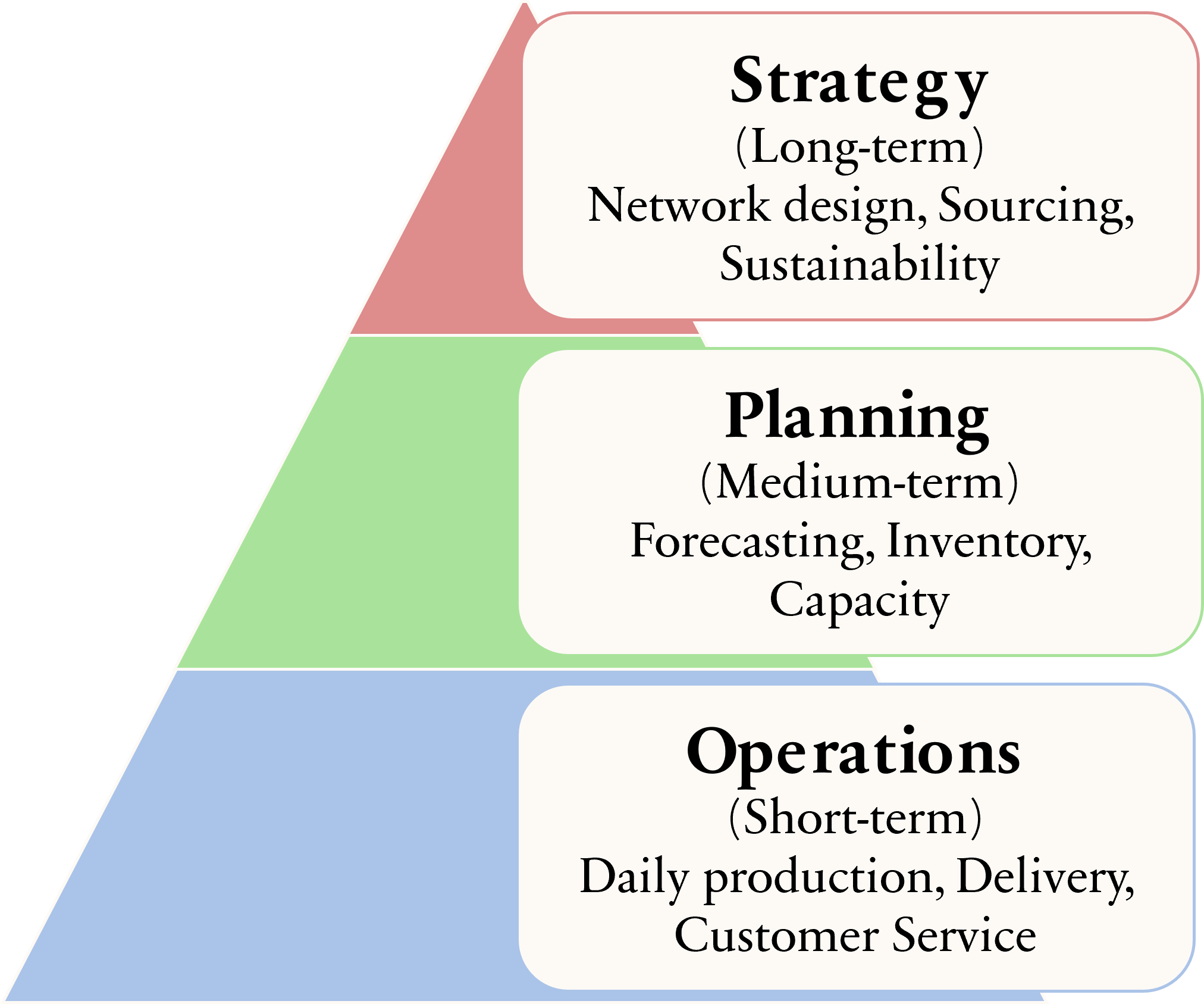
SCM links strategy, planning, and operations.

SCM Pyramid and Decision Levels

Push-Pull Strategy

The choice between push and pull strategies is fundamental to supply chain design.

Characteristic	Push	Pull	Hybrid
Demand Signal	Forecast	Actual	Mix
Inventory Location	Upstream	Downstream	Both
Lead Time	Longer	Shorter	Balanced
Flexibility	Lower	Higher	Moderate
Cost	Lower	Higher	Moderate
Pros	Economies of scale	Responsiveness	Balanced performance
Cons	Risk of overstock	Risk of stockouts	Complexity in management

PART II. NETWORK DESIGN

Deterministic Network Design
- Topic 2: single-echelon single-commodity (SESC).
- Topic 3: two-echelon multi-commodity (TEMC).

%%{init: {
  "flowchart": {
    "padding": 40,
    "nodeSpacing": 30,
    "rankSpacing": 100
  }
}}%%
flowchart LR
    DC1((" DC1 "))
    DC2((" DC2 "))
    C1((" C1 "))
    C2((" C2 "))
    C3((" C3 "))
    DC1 --> C1
    DC1 --> C2
    DC1 --> C3
    DC2 --> C1
    DC2 --> C2
    DC2 --> C3

Figure 1: SESC Model Example

%%{init: {
  "flowchart": {
    "htmlLabels": true,
    "padding": 40,
    "nodeSpacing": 25,
    "rankSpacing": 100
  }
}}%%
flowchart LR
    S1((" S1 "))
    S2((" S2 "))
    DC1((" DC1 "))
    DC2((" DC2 "))
    C1((" C1 "))
    C2((" C2 "))
    C3((" C3 "))

    S1 --> DC1
    S1 --> DC2
    S2 --> DC1
    S2 --> DC2
    DC1 --> C1
    DC1 --> C2
    DC1 --> C3
    DC2 --> C1
    DC2 --> C2
    DC2 --> C3

Figure 2: TEMC Model Example

Stochastic Network Design
- Topic 4: network design under uncertainty (DCF and NPV).

Topic 2: SESC Model

Set and Indices

$V_1$: potential facility locations
$V_2$: customer locations

$j \in V_1$: index for facilities
$k \in V_2$: index for customers

Parameters

$c_{jk}:$ transportation cost/unit
$f_j:$ fixed cost opening facility $j$

$d_k:$ customer $k$ demand
$K_j:$ facility $j$ capacity

Decision Variables

$y_{jk}:$ flow from facility $j$ to customer $k$
$z_j:$ binary variable indicating if facility $j$ is open

Objective

\[ \text{Minimise} \quad Z = \sum_{j \in V_1} \sum_{k \in V_2} c_{jk} y_{jk} + \sum_{j \in V_1} f_j z_j \]

Constraints

Demand satisfaction: $\sum_{j \in V_1} y_{jk} = d_k$ for all $k \in V_2$
Facility opening: $\qquad y_{jk} \leq K_j z_j$ for all $j \in V_1, k \in V_2$
Binary variables: $\quad\;\;\, z_j \in \{0,1\}$ for all $j \in V_1$
Non-negativity: $\qquad\; y_{jk} \geq 0$ for all $j \in V_1, k \in V_2$

Topic 3: TEMC Model

Sets and Indices

$V_0$: suppliers, $i \in V_0$
$V_1$: DCs, $j \in V_1$

$V_2$: customers, $k \in V_2$
$H$: commodities, $h \in H$

Parameters
- $c_{ijk}^h$: cost/unit from supplier $i$ to DC $j$ to customer $k$ for commodity $h$.
- $f_j$: fixed cost to open DC $j$.
- $g_j$: handling cost/unit at DC $j$.
- $D_k^h$: demand for commodity $h$ at customer $k$.
Decision Variables
- $x_{ijk}^h$: flow of commodity $h$ from supplier $i$ to DC $j$ to customer $k$.
- $y_{jk}$: total flow through DC $j$.
- $z_j$: binary variable indicating if DC $j$ is open.

Objective Function \[ \min Z = \sum_{i,j,k,h} c_{ijk}^h x_{ijk}^h + \sum_j\left(f_j z_j + g_j\sum_{k,h} D_k^h y_{jk}\right) \]
Constraints
- Demand satisfaction: $\sum_{i,j} x_{ijk}^h = D_k^h$ for all $k \in V_2, h \in H$.
- Flow conservation: $\quad y_{jk} = \sum_{i,h} x_{ijk}^h$ for all $j \in V_1, k \in V_2$.
- Facility opening: $\qquad y_{jk} \leq K_j z_j$ for all $j \in V_1, k \in V_2$.
- Binary variables: $\quad\;\;\, z_j \in \{0,1\}$ for all $j \in V_1$.
- Non-negativity: $\qquad\; x_{ijk}^h, y_{jk} \geq 0$ for all $i,j,k,h$.

SESC vs TEMC: Model Selection

Use SESC when:
- one commodity,
- single distribution echelon,
- faster MILP solve desired.
Use TEMC when:
- multi-product interactions matter,
- two-echelon structure is essential,
- handling capacities and product mix are important.

Deterministic Network Design Recap

Both models use binary location and continuous flow decisions.
Objective is still total cost minimisation.
Complexity increases with echelons and commodity count.

Topic 4: Network Design Under Uncertainty

Real systems include demand, supply, lead-time, and cost uncertainty.
Financial viability must be tested with discounted cash flows.
Decision trees and scenarios complement deterministic optimisation.

Present Value and NPV Formulas

\[ \boxed{PV_t = \frac{C_t}{(1+r)^t}} \qquad \boxed{NPV = C_0 + \sum_{t=1}^{T} \frac{C_t}{(1+r)^t}} \]

Cash flow in period $t, C_t$, discount rate $r$, $C_0$ is usually negative.
$NPV > 0$: value created, acceptable project.
$NPV = 0$: financial break-even.
$NPV < 0$: value destroyed, reject or redesign.
For alternatives, choose highest positive NPV under valid assumptions.

Decision Tree

Uncertainty in demand and/or price can be shown as branches with probabilities.
Depth of tree: number of sequential decisions or time periods. The following decision tree has a depth of 4 (4 sequential decisions or time periods).

%%{init: {
  "flowchart": {
    "padding": 40,
    "nodeSpacing": 25,
    "rankSpacing": 175
  },
  "themeVariables": {
    "fontSize": "22px"
  }
}}%%

flowchart LR

  P0(( )) --> |P1|P11(( ))
  P0 --> |P2|P12(( ))
  P0 --> |P3|P13(( ))

  P11 --> P21(( ))
  P11 --> P22(( ))
  
  P12 --> P22
  P12 --> P23(( ))
  P12 --> P24(( ))
  P12 --> P25(( ))

  P21 --> P31(( ))

  P22 --> P31
  P22 --> P32(( ))

  P23 --> P32
  P23 --> P33(( ))
  P23 --> P34(( ))

  P31 --> P41(( ))
  P31 --> P42(( ))

  P33 --> P43(( ))

  P34 --> P43(( ))
  P34 --> P44(( ))


  classDef default fill:#d1e7dd,stroke:#000000,color:#ffffff;

Calculate expected NPV at each node by rolling back from the leaves to the root, using probabilities and discounted cash flows.

Evaluating NPV: Bellman’s Principle

Solve the problem from the end (future outcomes) back to the beginning.

Structure the decision tree
- Draw nodes and terminal nodes (outcomes) connected with arrows
- Label branches with probabilities of occurrence.
Assign payoffs for each node
- For each node, calculate payoffs (profit) and state the probability.
Work backwards (Bellman’s principle)
- From the terminal node, calculate
  
  $\text{Expected Monetary Value (EMV)} = \sum (\text{Probability} \times \text{Payoff})$
- Discount EMV to Present Value (PV)
Continue working backward until you reach the initial decision.

PART III. FORECASTING TECHNIQUES

Forecasts align supply decisions with expected demand.
Better forecasts reduce stockouts and overstock.
Forecast horizon determines method and usable detail.

Forecast Horizons and Use Cases

Short-term: scheduling, replenishment, dispatching.
Medium-term: capacity planning, purchasing plans.
Long-term: strategic expansion and network redesign.

Demand Pattern Decomposition

\[ \text{Demand} = \text{Trend} + \text{Seasonality} + \text{Random Variation} \]

Level: stable base demand.
Trend: long-term in/decrease.

Seasonality: repeated periodic pattern.
Random: noise not captured by structure.

Topic 5. Demand Forecasting

Naive Forecast Baseline

\[ \boxed{F_{t+1} = F_t} \]

Useful as a benchmark.
Often weak when trend or seasonality is strong.

Moving Average ($n-$MA)

\[ \boxed{\hat{Y}_{t+1} = \frac{Y_t + \cdots + Y_{t-n+1}}{n}} \]

$n$ = number of periods
$\hat{Y}_{t+1}$ = forecast for the next period

Weighted Moving Average ($n-$WMA)

\[\boxed{\hat{Y}_{t+1} = w_1Y_t + \cdots + w_nY_{t-n+1}}\]

$\sum w_i = 1$
Assign more weight to recent data for responsiveness.

Simple Exponential Smoothing ($\alpha$-SES)

\[\boxed{\hat{Y}_{t+1} = \alpha Y_t + (1 - \alpha)\hat{Y}_t}\]

$\alpha$ smoothing constant ($0 < \alpha \leq 1$)
$Y_t$ actual value at time $t$
$\hat{Y}_t$ forecast for time $t$

Linear Regression Forecasting

\[ \boxed{\hat{y} = a + bx}\;\;\boxed{b = \frac{\Delta y}{\Delta x}} \] \[ SSE = \sum (y_i - \hat{y}_i)^2 \]

Choose coefficients to minimise SSE.
Interpret residuals for model adequacy.

\[\boxed{b = \frac{\sum XY - n\bar{x}\bar{y}}{\sum X^2 - n\bar{x}^2} = \frac{\sum (X_i - \bar{x})(Y_i - \bar{y})}{\sum (X_i - \bar{x})^2}}\]

\[\boxed{a = \bar{y} - b\bar{x}, \quad \bar{x} = \frac{\sum X}{n}, \quad \bar{y} = \frac{\sum Y}{n}}\]

Multiple Regression Forecasting

\[ \boxed{\hat{y} = a + b_1x_1 + b_2x_2 + \cdots + b_kx_k} \]

Forecast depends on multiple independent variables $x_1, x_2, \ldots, x_k$.
Usually solved with matrix algebra or software for coefficient estimation.
In the case of two independent variables, $\hat y = a + b_1x_1 + b_2x_2$, the coefficients can be estimated using the following system of equations derived from the least squares method:

\[ \boxed{ \begin{align} \sum Y =&\;\; na + b_1 \sum X_1 + b_2 \sum X_2 \\ \\ \sum X_1Y =&\;\; a \sum X_1 + b_1 \sum X_1^2 + b_2 \sum X_1X_2\\ \\ \sum X_2Y =&\;\; a \sum X_2 + b_1 \sum X_1X_2 + b_2 \sum X_2^2 \end{align} } \]

Evaluation Metrics

Other than the sum of squared errors (SSEs), there are several metrics to evaluate the accuracy of forecasting models. Common ones include:

Metric	Formula	Interpretation
Sum of Absolute Errors (SAE)	$\sum \|y_i - \hat{y}_i\|$	Total absolute error between actual and forecasted values. Lower is better.
Mean Absolute Error (MAE)	$\dfrac{1}{n} \sum \|y_i - \hat{y}_i\|$	Average absolute error between actual and forecasted values. Lower is better.
Root Mean Squared Error (RMSE)	$\sqrt{\dfrac{1}{n} \sum (y_i - \hat{y}_i)^2}$	Square root of average squared error. More sensitive to large errors. Lower is better.
Mean Absolute Percentage Error (MAPE)	$\dfrac{100\%}{n} \sum \left\| \dfrac{y_i - \hat{y}_i}{y_i} \right\|$	Average absolute percentage error. Useful for comparing across different scales. Lower is better.
R-squared ($R^2$)	$1 - \dfrac{\sum (y_i - \hat{y}_i)^2}{\sum (y_i - \bar{y})^2}$	Proportion of variance in the dependent variable explained by the model. Higher is better (max 1).

PART IV. INVENTORY MODELS & CONTROL STRATEGIES

Core decision pair: how much to order and when to reorder.

Deterministic models assume known demand and lead time, leading to closed-form solutions like EOQ or EPQ.
- EOQ: Economic Order Quantity for discrete orders.
  - Determines optimal order size to minimise total cost.
- EPQ: Economic Production Quantity for continuous production.
  - Determines optimal production batch size when items are produced and consumed simultaneously.
Stochastic models account for demand and/or lead time variability, requiring safety stock and service level considerations.
- Continuous review (Q,R): order $Q$ when inventory position hits $R$.
- Periodic review (P): review every $P$ and order up to a target level.
- Newsvendor model: single-period inventory decision.

Common Notations

Notation	Unit	Description
$C$	$/unit	Purchase or manufacturing cost of an item
$A$ or $K$	$/order	The ordering cost per order
$I$	%	Inventory carrying cost rate or interest rate
$h$	$/unit/time	Inventory holding cost of an item per unit per time unit
$k$	$/unit/time	Shortage cost per unit short per time
$D$	units/year	Demand rate per planning horizon per year
$d$	units/time	Demand rate per time unit (e.g., per day)
$r$	units/time	Production rate (for EPQ)
$S$	units	Shortage quantity, a decision variable
$Q$	units	Order quantity, a decision variable
$T$	Time	Cycle time (time between orders), a decision variable
$R$	units	Reorder level (inventory level at which an order is placed)
$L$	Time	Lead time

Topic 6. Deterministic Inventory Models (EOQ & EPQ)

Economic Order Quantity (EOQ)

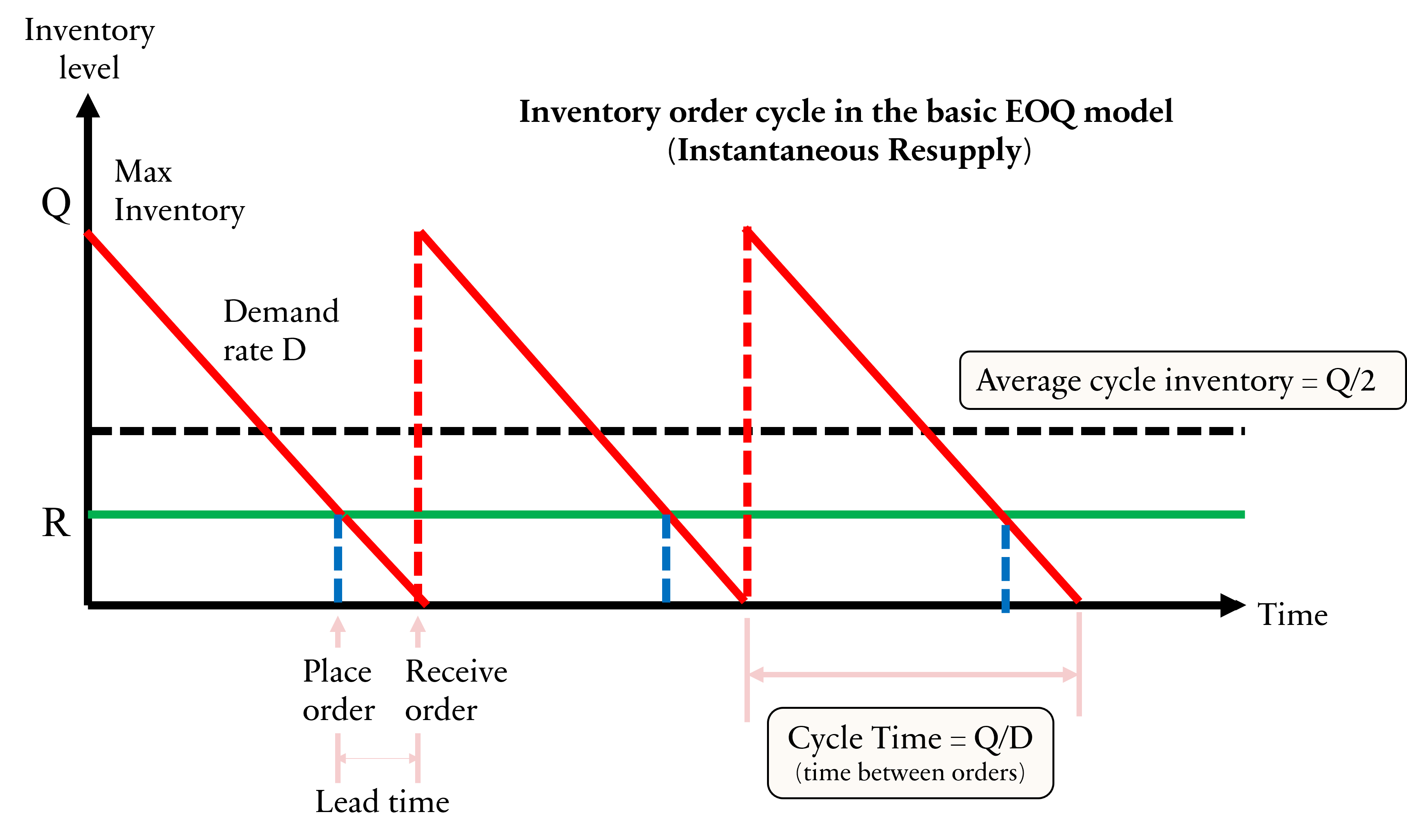
Basic EOQ Core Formula

\[ \boxed{Q^* = \sqrt{\frac{2DA}{h}}} \quad \boxed{OC = \frac{DA}{Q^*}} \quad \boxed{IHC = \frac{Q^*h}{2}} \]

\[ \boxed{TC = \frac{DA}{Q^*} + \frac{Q^*h}{2} = \sqrt{2DAh}} \]

\[ \boxed{T = \frac{Q^*}{D}} \quad \boxed{\text{Order Frequency} = \frac{D}{Q^*}} \]

\[ \boxed{\frac{TC(Q_1)}{TC(Q^*)} = \frac{1 + b^2}{2b}} \quad \text{where } Q_1 = bQ^* \]

EOQ with Shortage

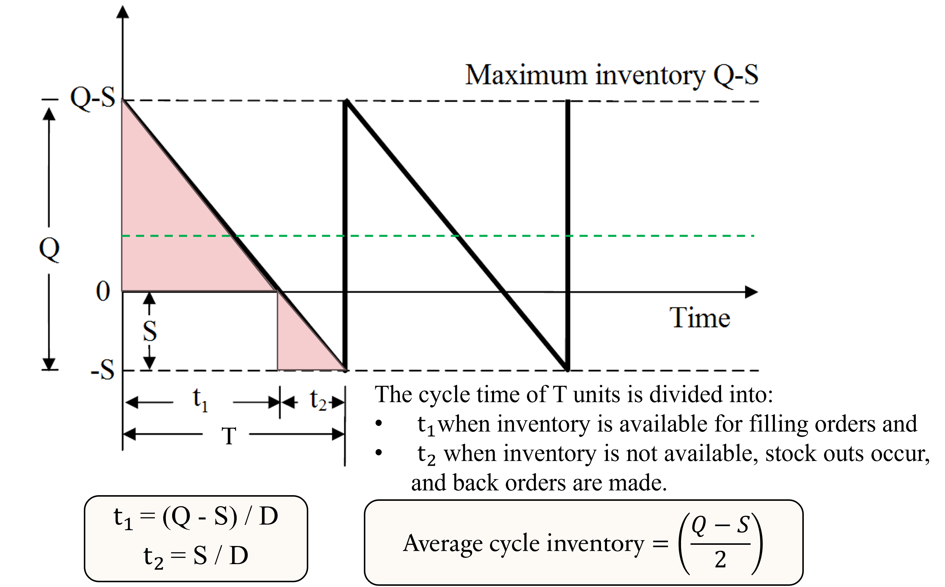
EOQ with Shortage Formula

\[ \boxed{Q^* = \sqrt{\frac{2DA}{h}\frac{k+h}{k}}} \quad \boxed{S^* = Q^*\frac{h}{k+h}} \quad \boxed{Q^* - S^* =Q^*\frac{k}{k+h}} \]

\[ \boxed{IHC = \frac{(Q^* - S^*)^2}{2Q^*} \cdot h} \quad \boxed{SC = \frac{(S^*)^2}{2Q^*} \cdot k} \]

\[ \boxed{TC^* = \frac{DA}{Q^*} + \frac{(Q^* - S^*)^2}{2Q^*} \cdot h + \frac{(S^*)^2}{2Q^*} \cdot k = \sqrt{2DSAh\frac{k}{k+h}}} \]

Economic Production Quantity (EPQ)

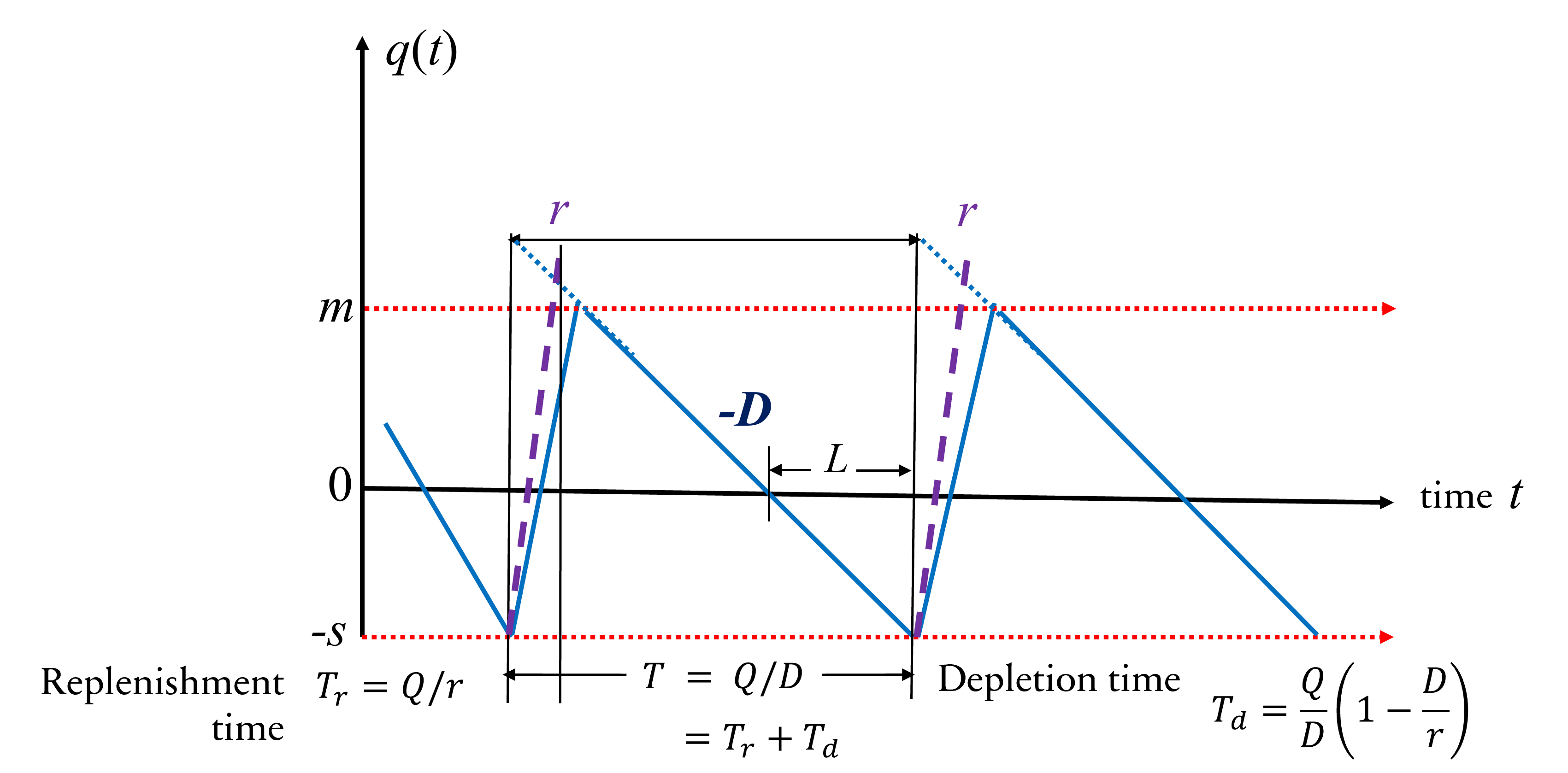
EPQ Core Formula

\[ \boxed{Q^* = \sqrt{\frac{2DA}{h}\frac{r}{r-D}} = \sqrt{\frac{2DA}{h(1-D/r)}}} \]

\[ \boxed{T = \frac{Q^*}{D} = T_r + T_d} \quad \boxed{T_r = \frac{Q^*}{r}} \quad \boxed{T_d = \frac{Q^*}{D}\left(1 - \frac{D}{r}\right)} \]

\[ \boxed{I_{max} = Q^*\left(1 - \frac{D}{r}\right)} \quad \boxed{IHC = \left(1 - \frac{D}{r}\right)\frac{Q^*}{2}h} \]

\[ \boxed{TC^* = \frac{DA}{Q^*} + \left(1 - \frac{D}{r}\right)\frac{Q^*}{2}h = \sqrt{2DAh\left(1 - \frac{D}{r}\right)}} \]

Topic 7. Inventory with Quantity Discounts and Multi-Commodity

Supplier lowers unit price for larger purchases.
Benefit: lower purchase cost.
Risk: higher average inventory and carrying cost.

Discount Types

All-units discount: one price tier applies to all units in the order.
Incremental discount: lower tier price applies only to units above breakpoint.

Multi-commodity Inventory Models

Aggregating multiple products in a single order
Lot sizing with multiple products or customers
- Delivered independently for each product
- Delivered jointly for all products
- Delivered jointly for a selected subset of the products

EOQ with All-Units Discount

For each discount breaks $q_i$, compute the EOQ as if that price applied to all units, then evaluate total cost at that EOQ.

\[ \boxed{Q_i^* = \sqrt{\frac{2DA}{IC_i}}} \quad \boxed{\hat{Q}_i = \begin{cases} q_i, & Q_i^* < q_i \\ Q_i^*, & q_i \le Q_i^* \le q_{i+1} \\ q_{i+1}-1, & Q_i^* > q_{i+1} \end{cases}} \]

\[ \boxed{TC_i(Q) = C_iD + \frac{D}{Q}A + \frac{Q}{2}h_i} \quad \boxed{h_i = IC_i} \]

\[ \boxed{Q^* = \arg\min_i TC_i(\hat{Q}_i)} \]

Tips: Starting from the cheapest unit price tier, check if the EOQ falls within that tier. If not, move to the next tier until you find a feasible EOQ or reach the last tier.

EOQ with Incremental Discount

For a discount break $q_j$, the optimal order quantity $Q_j^*$:

\[ \boxed{Q_j^* = \sqrt{\frac{2(R_j-C_jq_j+A)d}{IC_j}}} \\ \boxed{R_j= C_1(q_2-q_1)+C_2(q_3-q_2)+\ldots+C_{j-1}(q_j-q_{j-1})} \\ \boxed{C(Q)=R_j +C_j(Q-q_j)} \\ \boxed{ TC(Q_j) = \frac{C(Q_j)}{Q_j}d+\frac{D}{Q_j}A+\frac{Q_j}{2}(I\times \frac{C(Q_j)}{Q_j}) } \]

Tips: Compute $Q_j^*$ for each discount break $q_j$. Disregard any $Q_j^*$ that is not feasible (i.e., does not satisfy the discount break condition). For each feasible $Q_j^*$, compute the total cost. Choose the $Q_j^*$ that yields the lowest total cost.

Multi-Commodity Inventory Models

Aggregating $n$ products in a single order

Independent demand, fixed ordering cost, and the same holding cost.

\[ \boxed{T^*=\sqrt{\frac{2A}{h\sum_{i=1}^n D_i}}} \]

Independent demand, fixedordering cost, and different holding cost rates.

\[ \boxed{T^*=\sqrt{\frac{2A}{\sum_{i=1}^n D_i h_i}}} \]

Independent demand, fixed ordering cost plus product-specific fixed costs $A_i$, and different holding cost rates.

\[ \boxed{T^*=\sqrt{\frac{2(A+\sum_{i=1}^n A_i)}{\sum_{i=1}^n D_i h_i}}} \]

Use the optimal cycle time $T^*$,

\[ \boxed{Q_i^* = D_i T^*} \]

$\boxed{TC^* = \sqrt{2\left(A+\sum_{i=1}^n A_i\right)\sum_{i=1}^n D_i h_i}}$

Lot sizing with multiple products or customers

Delivered independently for each product

\[ \boxed{Q_i^* = \sqrt{\frac{2DA}{h_i}}} \quad \boxed{TC^* = \sum_{i=1}^n \left(\frac{D}{Q_i^*}A + \frac{Q_i^*}{2}h_i\right) = \sum_{i=1}^n \sqrt{2DAh_i}} \]

Delivered jointly for all products

\[ \boxed{n^* = \sqrt{\frac{\sum_{i=1}^k D_i I C_i}{2A^*}}} \quad \boxed{A^* = A + \sum_{i=1}^n A_i} \quad \boxed{Q_i^* =\frac{D_i}{n^*}} \]

\[ \boxed{\text{OC}= n^*A^*} \quad \boxed{\text{IHC}= \frac{1}{2n^*}\sum_{i=1}^n D_i I C_i} \quad \boxed{TC(n^*)=OC +IHC} \]

Delivered jointly for a selected subset of the products

\[ \boxed{\overline{n}_i = \sqrt{\frac{IC_iD_i}{2(A+A_i)}}} \quad \boxed{\overline{n}=\max \{\overline{n}_i\}} \quad \boxed{\overline{\overline{n}}_i = \sqrt{\frac{IC_iD_i}{2 A_i}}} \]

\[ \boxed{\overline{m}_i=\overline{n}/\overline{\overline{n}}_i} \quad \boxed{m_i = \lceil \overline{m}_i \rceil} \]

\[ \boxed{n = \sqrt{\frac{\sum IC_i m_i D_i}{2[A+\sum (A_i/m_i)]}}} \quad \boxed{n_i = \frac{n}{m_i}} \]

\[ \boxed{Q_i^* = D_i/n_i} \]

\[ \boxed{TC = n \left[A + \sum_i \frac{A_i}{m_i}\right] + \frac{1}{2n}\sum_i IC_iD_im_i} \]

Topic 8. Stochastic Inventory Control Policies

Deterministic assumptions fail under random demand/lead time.
Safety stock is used to achieve target service levels.

(Q,R) vs P Policy: Quick Comparison

Characteristic	(Q,R) Policy	P Policy
Review	Continuous	Periodic (every P time units)
Order Quantity	Fixed (Q)	Variable (up to target level)
Reorder Point	R (when inventory position hits R)	N/A (orders placed at fixed intervals)
Responsiveness	High (reacts immediately to demand)	Lower (reacts only at review times)
Safety Stock	Typically lower (due to continuous monitoring)	May require more (to cover between reviews)
Monitoring Effort	Higher (requires constant tracking)	Lower (only at review times)
Coordination	More complex (as orders can occur at any time)	Simpler (orders occur at fixed intervals)

Continuous Review (Q,R) Policy

Constant Demand & Lead Time

\[ \boxed{R = d \times L} \\ \boxed{R = d \times L - n \times Q^*} \]

If $L>T$, $n=\lfloor L/T \rfloor$

Variable Demand & Constant Lead Time

\[ \boxed{ROP = \bar{d}L + SS} \\ \boxed{SS = z\sigma_d\sqrt{L}} \]

$z=\Phi^{-1}(\text{Service Level})$

Constant Demand & Variable Lead Time

\[ \boxed{R = d\bar{L} + SS} \\ \boxed{SS = zd\sigma_{LT}} \]

Variable Demand & Variable Lead Time

\[ \boxed{ROP = \bar{d}\bar{L} + SS} \\ \boxed{SS = z\sqrt{\bar{L}\sigma_d^2 + \bar{d}^2\sigma_{LT}^2}} \]

Periodic Review (P) Policy

Uncertainty	Safety Stock (SS)	Order-Up-To Level (TIL)
No	$0$	$d(P+L)$
Demand only	$z\sigma_d\sqrt{P+L}$	$\bar d(P+L)+SS$
Lead time only	$zd\sigma_{LT}$	$d(P+\bar L)+SS$
Both	$z\sqrt{\sigma_d^2(P+\bar L)+\bar d^2\sigma_{LT}^2}$	$\bar d(P+\bar L)+SS$

If using the EOQ-based optimal review peiod $T$, then replace $P$ with $T$ in the above formulas to get $I_\max.$

\[ \boxed{T=\frac{Q^*}{\bar d}=\sqrt{\frac{2K}{\bar d h}}} \quad \boxed{I_{\max}=TIL} \\ \boxed{\text{Protection Period} = P + \bar L \text{ or } T + \bar L} \\ \boxed{TIL = \text{Expected demand during } (P+\bar L) + \text{Safety Stock}} \]

Newsvendor Model (Single-Period Normal-Demand)

Single period inventory decision under demand uncertainty.
Balance overstock and understock costs to find optimal order quantity.

\[ \boxed{C_o = c-u} \quad \boxed{C_u = r-c} \quad \boxed{CR = \frac{C_u}{C_u + C_o} = \frac{r-c}{r-u}} \]

Higher $CR$ means understocking is more costly, so you want to order more.
Lower $CR$ means overstocking is more costly, so you want to order less

\[ \boxed{P(D \le Q^*) = CR} \quad \boxed{Q^* = \mu + z\sigma, \quad \Phi(z)=CR} \]

Choose the order quantity $Q^*$ such that the probability of demand being less than or equal to $Q^*$ equals the critical ratio.

Expected total cost for order quantity $Q$

Expected total cost includes expected overstock cost and expected understock cost, weighted by their respective probabilities.

\[ \boxed{E[TC(Q)] = C_oE[(Q-D)^+] + C_uE[(D-Q)^+]} \\ \boxed{E[(Q-D)^+] = \sigma[\phi(z)+z\Phi(z)]} \\ \boxed{E[(D-Q)^+] = \sigma[\phi(z)-z(1-\Phi(z))]} \\ \boxed{z = \frac{Q-\mu}{\sigma}} \]

Uncertainty	Safety Stock (SS)	Order-Up-To Level (TIL)
No	\(0\)	\(d(P+L)\)
Demand only	\(z\sigma_d\sqrt{P+L}\)	\(\bar d(P+L)+SS\)
Lead time only	\(zd\sigma_{LT}\)	\(d(P+\bar L)+SS\)
Both	\(z\sqrt{\sigma_d^2(P+\bar L)+\bar d^2\sigma_{LT}^2}\)	\(\bar d(P+\bar L)+SS\)