STAT2005 Computer Simulation

Lecture 1 — Introduction to Computer Simulation

Sam Wiwatanapataphee (275287a@curtin.edu.au)

19 Feb 2026

Goals today

  • Unit Information
  • Blackboard Tour
  • Lecture 1: Introduction to computer simulation
    • 1.1 What is Simulation?
    • 1.2 Simulation Workflow
    • 1.3 Simulation vs Analytical Solutions
    • 1.4 Random Number Generation (LCGs, Uniform)
    • 1.5 Revision: Probability Tools for Simulation

Unit Information


Unit Learning Outcomes

On successful completion of this unit you are expected to:

  1. explain the scope and limitation of simulation;
  2. develop simulation procedures in an appropriate computing environment;
  3. analyse and interpret simulation result;
  4. apply simulation techniques in a discipline specific context.


Learning Activities

  • Lecture (F2F, live via iLecture):
    • Thursday 10am – 12pm at 201.412
  • Workshop (F2F, live via MS Team, start in Week 1):
    • Thursday 12pm – 2pm at 312.222
  • Please bring your own device to both sessions.

Assessments

Task Value Due
Computer-based test 20% Week 5 & 11
Project 30% Week 6 & 14
Final Exam 50% Week 16 – 17


  • More details will be posted on BB.


Programming Language

  • R (required; assessed)
  • Python (optional; not assessed)
  • Choose either R or Python to complete the project.

Blackboard Tour

Lecture 1: Introduction to Computer Simulation

In the mid-1940s…

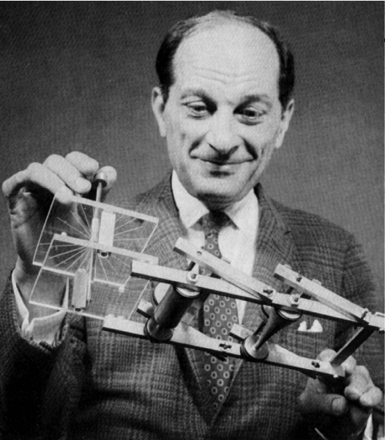
Stanisław Ulam

“What is the probability that a solitaire game can be won?”

“Why not just play a thousand times and count how often I win?”

John Von Neumann
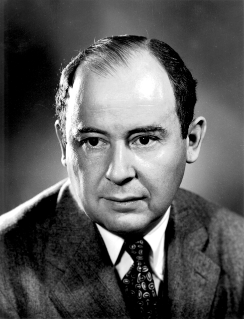
“If we can solve solitaire this way, we can solve anything this way.”

  • Humans can’t repeat a process thousands of times quickly enough.
  • Machines can.

ENIAC

(Electronic Numerical Integrator and Computer)

Together, Ulam and von Neumann developed a new method:

  • simulate randomness
  • repeat the process thousands of times
  • let the pattern emerge from noise
  • They named it Monte Carlo, after the famous casino.
1.1 What is Simulation?

Science and engineering are based on three pillars:

Observations

Experimentation

Computation

Measure and record real outcomes

Try experimenting with different assumptions (priors)

Simulate many possible scenarios to see what’s likely

Simulation is using a computer to imitate a real-world random process in order to learn about its behaviour.

It is a way of doing experiments when real experiments are expensive, slow, or impossible.

What can be simulated? Many coin tosses, customer arrivals in a shop, rainfall over a year, the lifetime of a machine/battery, the decaying of a radioactive source, etc.

Simulation = model + randomness + repetition

  • A model of the process
  • Randomness to reflect uncertainty
  • Repetition to understand variability

Simulation is systematic, follows explicit rules, and produces reproducible results.

1.2 Simulation Workflow

If simulation is an experiment on a computer, then we need to ask:

  • How do we design the experiment?
  • How do we run it?
  • How do we learn from the results?
Problem
Model
Simulation
Analysis
Conclusion

Examples: How long will customers wait in a coffee-shop queue?

  • “If customers arrive randomly, how long will they wait in line?”
  • “Do I need a second barista during busy hours?”
  • Customers arrive according to a random process (e.g., exponential inter‑arrival times).
  • Service times are also random (e.g., normally or exponentially distributed).
  • There is one barista (one server)
  • Customers form a single queue.
  • This is a queueing model – a classic simulation setup
  • Generate random arrival times and random service times
  • Track the queue length over time
  • Record each customer’s waiting time
  • Repeat for thousands of simulated hours
  • Average and maximum waiting time
  • Distribution of waiting times
  • Probability that the queue exceeds 5 people
  • Comparison between one‑barista vs two‑barista scenarios
  • Visualisation: histograms, time‑series plots, boxplots.
  • With one barista, average wait = 6 minutes, and long queues occur 30% of the time.
  • With two baristas, average wait = 3 minutes, and long queues almost never form.
  • Recommendation: add a second barista during peak hours.

The simulation answers the original question.
%%{init: {'flowchart': {'nodeSpacing': 10, 'rankSpacing': 10}}}%%
flowchart TB
  A[Formulate<br/>problem] --> B[Data &<br/>Assumption] --> C([Assumptions<br/>OK?])
  C -->|Yes| D[ Program<br/>model] --> E([Model<br/>OK?])
  E -->|Yes| F[Analyse] --> G[Conclusion]

  C -->|No| R((Revise))
  E -->|No| R
  R --> A
  R --> B

Designing a Simulation Study Flowchart

Key idea

  • Simulation studies are iterative
  • Validation happens early and often
  • Revision is normal, not failure

Example Queueing system

  1. Problem: Wait time, service time
  2. Data & Assumption: Arrival rates, service times, single queue, identical agents
  3. Assumptions OK? Poisson or constant arrivals? Heavy-tailed service times?
  4. Model: Discrete-event simulation
  5. Model OK? Code correctness, matches reality
  6. Analyse: Performance measures, CIs, visualise
  7. Conclusion: Recommendations, expected improvement, limitations, and next steps

“Simulation is not magic.”

“Simulation is not magic.”

Garbage in → garbage out

If the model is wrong,
the results will be wrong.

Model assumptions matter

Every simulation depends on:

  • assumptions about randomness
  • assumptions about structure
  • assumptions about parameters

Simulation approximates

Simulation produces:

  • estimates

  • variability

  • uncertainty

  • Never exact answers.

1.3 Simulation vs Analytical Solutions

Simulation and analytical solutions are two different ways of answering scientific or engineering questions. They often aim at the same goal, but they work in fundamentally different ways and shine in different situations.

Analytical solutions
  • Formulas/exact, showing how variables relate
  • Strong assumptions
  • Often elegant and fast to compute
When to use
  • The system is simple enough to model with equations
  • The mathematics is tractable
  • You need exact results
  • You want to understand the structure of the problem
Example

For a simple queue with arrival rate \(\lambda\) and service rate \(\mu,\) the average number of customers in the system is:

\[ L=\frac{\lambda }{\mu -\lambda } \]

Simulation
  • Produces approximate answers
  • Handles complex, realistic systems
  • Requires computational power
  • Flexible: you can model almost anything
When to use
  • The system is too complicated for closed‑form math
  • You want to include realistic randomness
  • You want to test “what‑if” scenarios
  • You need distributions, not just averages
Example

If the café has:

  • two baristas with different speeds
  • customers who sometimes abandon the queue
  • peak and off‑peak arrival patterns
  • priority customers (e.g., mobile orders)

A simple side-by-side example

Question Analytical Simulation
“What’s the probability of getting exactly 7 heads in 10 flips?” Use binomial formula: \(\dbinom{10}{7}0.5^{10}\) Simulate 10,000 sets of 10 flips and count how often 7 heads appear
“What’s the distribution of waiting times in a complex queue?” No closed‑form solution Simulate arrivals and service events many times
“How does changing a parameter affect the system?” Differentiate the formula Re‑run the simulation with new parameters


Comparison

Analytical Simulation
Exact (if possible) Approximate
Requires tractable math Requires computation
Fast once derived Slower, but flexible
Limited by assumptions Handles complexity


Simulation trades exactness for generality and understanding. To simulate anything, we need randomness, control over randomness, and reproducibility.

This brings us to random number generation.

1.4 Random Number Generation

True Randomness

True randomness comes from physical processes that are inherently unpredictable.

Example
radioactive decay thermal noise atmospheric noise
quantum events rolling a real die flipping a real coin

These processes have no underlying pattern. If you repeat them, you cannot predict the next outcome, even in principle.

True randomness is non‑deterministic.


Pseudorandom \(\neq\) Random

Computers do not generate truly random numbers. They use pseudorandom number generators (PRNGs)

  • starts with a seed
  • applies a deterministic formula
  • produces a long sequence of numbers that look random
  • but are fully reproducible (if using the same seed)
Pseudorandom numbers are deterministic randomness.

1.4.1 Linear Congruential Generators (LCGs)

LCGs are the simplest and most historically important PRNGs. They were used in early Monte Carlo simulations. It is easy to implement, fast, and memory-light. An LCG produces a sequence of integers using a recurrence relation:

\[ X_{n+1} = (aX_n + c) \mod m, \]

where \(X\) is the sequence of pseudo-random values and

  • the modulus \(m, 0 < m\)
  • the multiplier \(a, 0 < a < m\)
  • the increment \(c, 0 \leq c < m\)
  • the seed or start values \(X_0, 0 \leq X_0 < m\)

lcg <- function(n, seed = 1, a = 1664525, c = 1013904223, m = 2^32) {
  x <- numeric(n)
  x[1] <- seed
  for (i in 2:n) {
    x[i] <- (a * x[i-1] + c) %% m
  }
  return(x)
}
set.seed(123)
u <- lcg(1000); head(u)
[1]          1 1015568748 1586005467 2165703038 3027450565  217083232

An LCG produces integers, and the range of those integers is determined entirely by the choice of parameters \(a, c,\) and especially \(m.\) These integer are always between 0 and \(m-1.\)

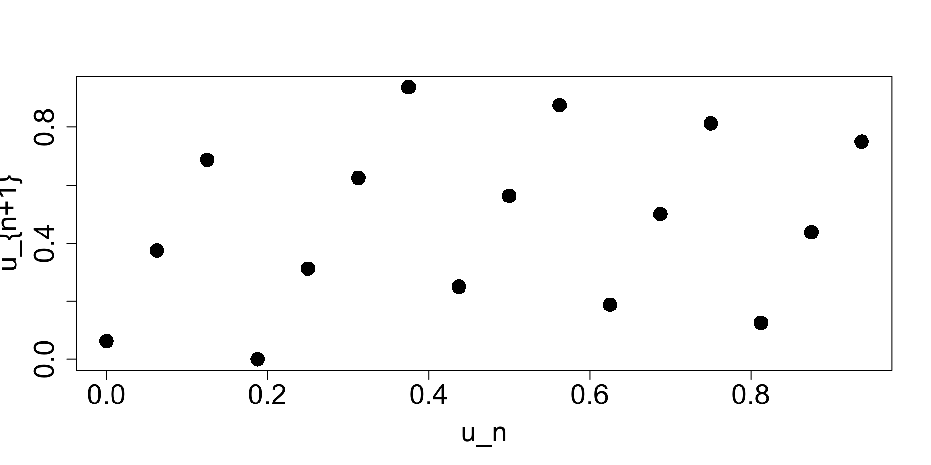
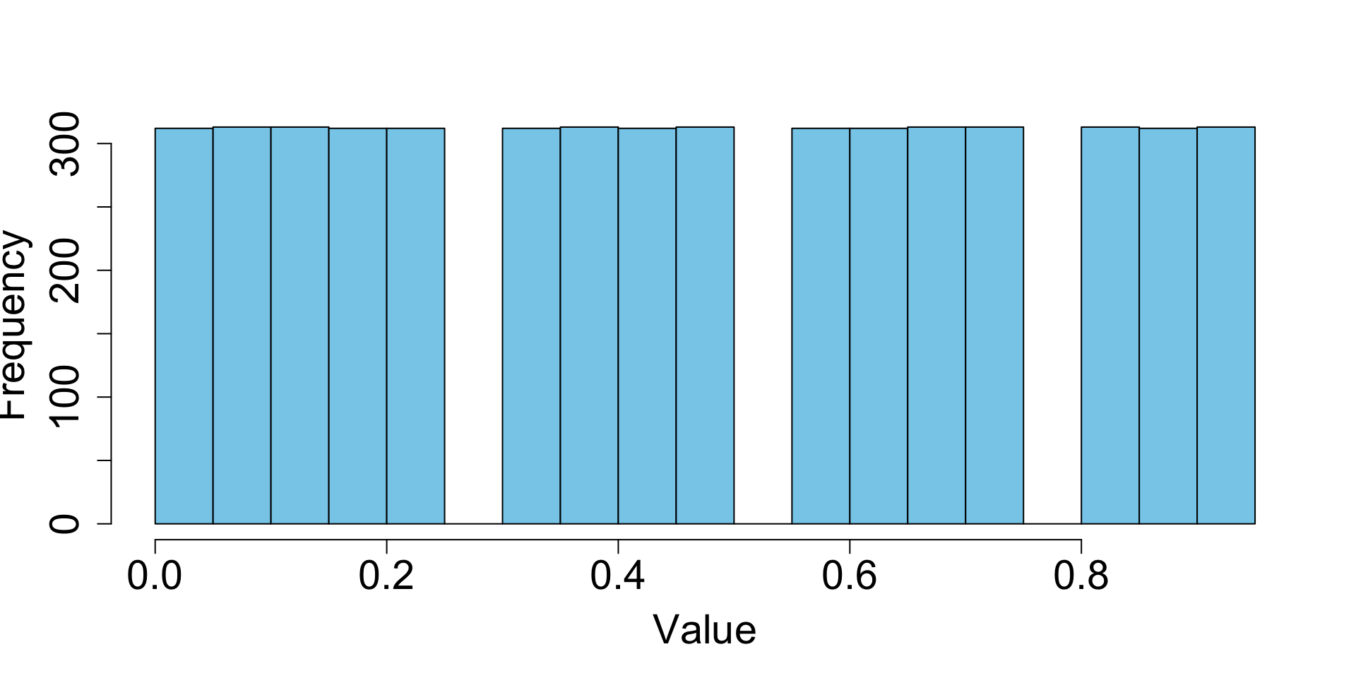
# Bad LCG
lcg <- function(n, seed = 1, a = 5, c = 1, m = 16) {
  x <- numeric(n)
  x[1] <- seed
  for (i in 2:n) {
    x[i] <- (a * x[i-1] + c) %% m
  }
  u <- x / m   # convert to Uniform(0,1)
  return(u)
}
set.seed(123); u <- lcg(5000)
hist(u, breaks=30, col="skyblue",
     xlab="Value", main="",
     cex.axis=1.8, cex.lab=1.8)

plot(u[-5000], u[-1], pch=16, cex=2, 
    xlab = "u_n", ylab = "u_{n+1}",
    cex.axis=1.8, cex.lab=1.8)

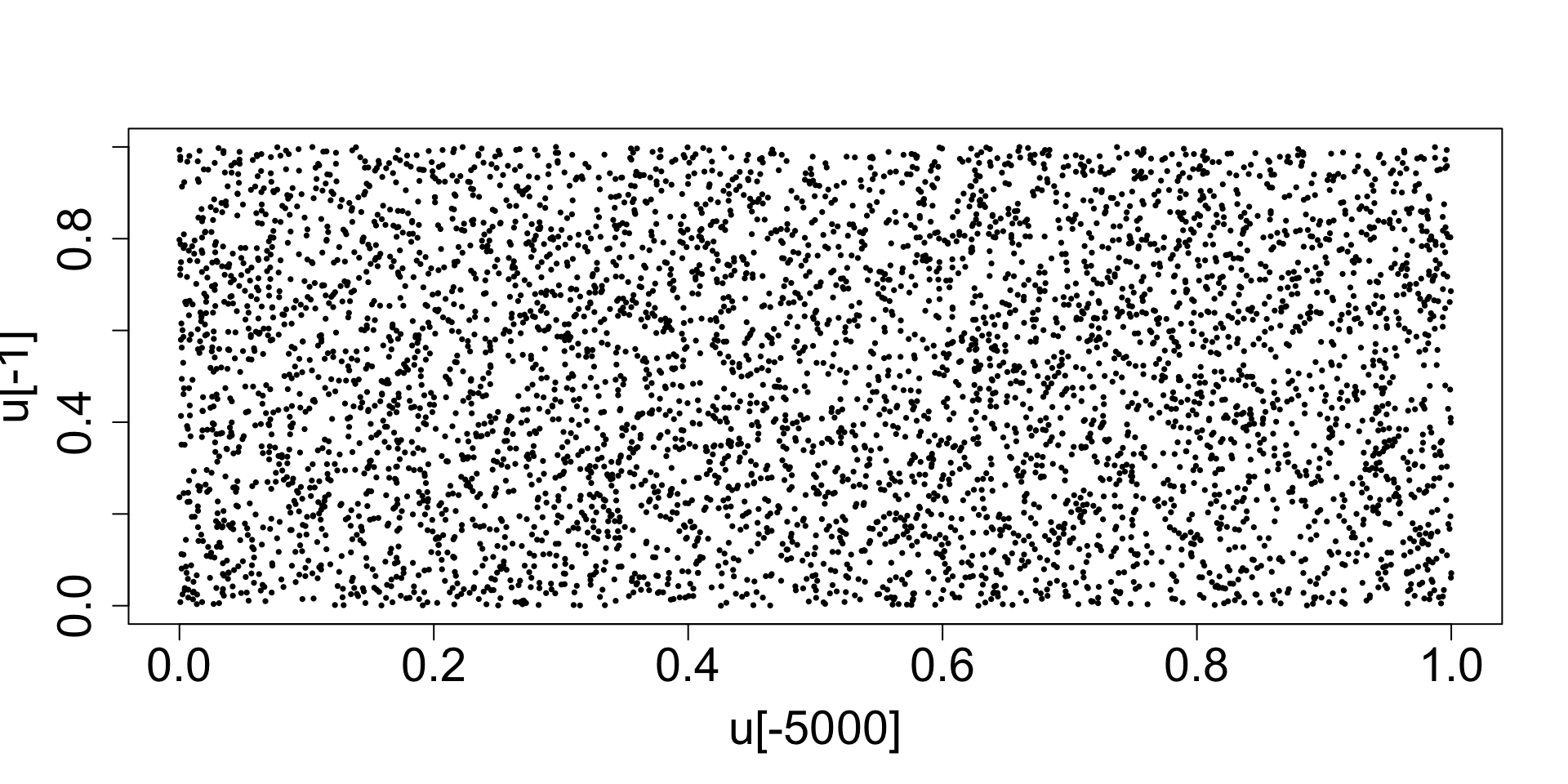
The nature of modulo arithmetic means the sequence will eventually repeat itself. Therefore, LCGs have structural weaknesses: short periods, visible lattice patterns, poor performance in high-dimensional simulations.

# Good LCG
lcg <- function(n, seed, a, c, m, as.uniform = TRUE) {
  x <- numeric(n)
  x[1] <- seed
  for (i in 2:n) {
    x[i] <- (a * x[i - 1] + c) %% m
  }
  if (as.uniform) {
    return(x / m)   # convert to Uniform(0,1)
  } else {
    return(x)       # return raw integers
  }
}
set.seed(123); u <- lcg(n=5000, seed=1, a=1664525, c=1013904223, m=2^32)
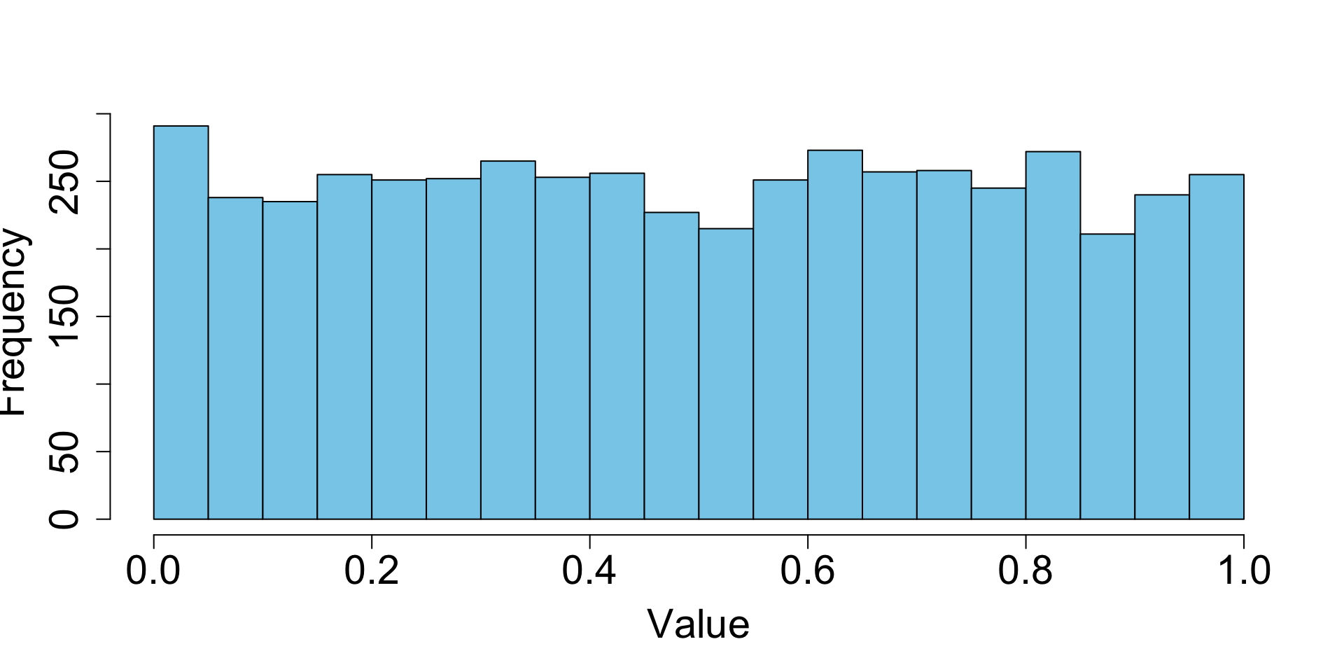
hist(u, breaks=30, col="skyblue",
    main="", xlab="Value",
    cex.axis=1.8, cex.lab=1.8)

# Successive pair plot
plot(u[-5000], u[-1], pch=16, cex=0.5,
    cex.axis=1.8, cex.lab=1.8)

1.4.2 Uniform(0,1) Random Number (Mersenne Twister)

Mersenne Twister is the modern default pseudorandom number generator in R, Python, NumPy, MATLAB, Julia, and many other systems. It’s designed to produce high‑quality Uniform(0,1) values for simulation.

\[ U \sim Uniform(0,1) \]

  • Equally likely takes values between 0 and 1
  • Imagine repeatedly picking a point at random on the interval (0,1) for a thousand time.
  • Over many draws, the points spread out evenly
set.seed(123); u <- runif(1000, 0, 1)

Why Uniform(0,1) is important?

Because if you can generate high‑quality Uniform(0,1) values, you can transform them into any other distribution!

Bernoulli(p)

Generate \(U \rightarrow\) If \(U < p\), return 1, else return 0

Exponential(\(\lambda\))

Use the inverse CDF: \(\qquad X=-\frac{1}{\lambda }\ln (1-U)\)

Normal(0,1)

Use the Box–Muller transform: \(\qquad Z=\sqrt{-2\ln U_1}\, \cos (2\pi U_2)\)

Every simulation — from Ulam’s solitaire experiments to modern Bayesian MCMC — relies on the ability to generate random draws. The workflow is always

  • Start with Uniform(0,1)
  • Transform it into the distribution you need
  • Use those draws to simulate the system
  • Repeat thousands of times
“if you can simulate randomness, you can solve problems too hard for equations.”
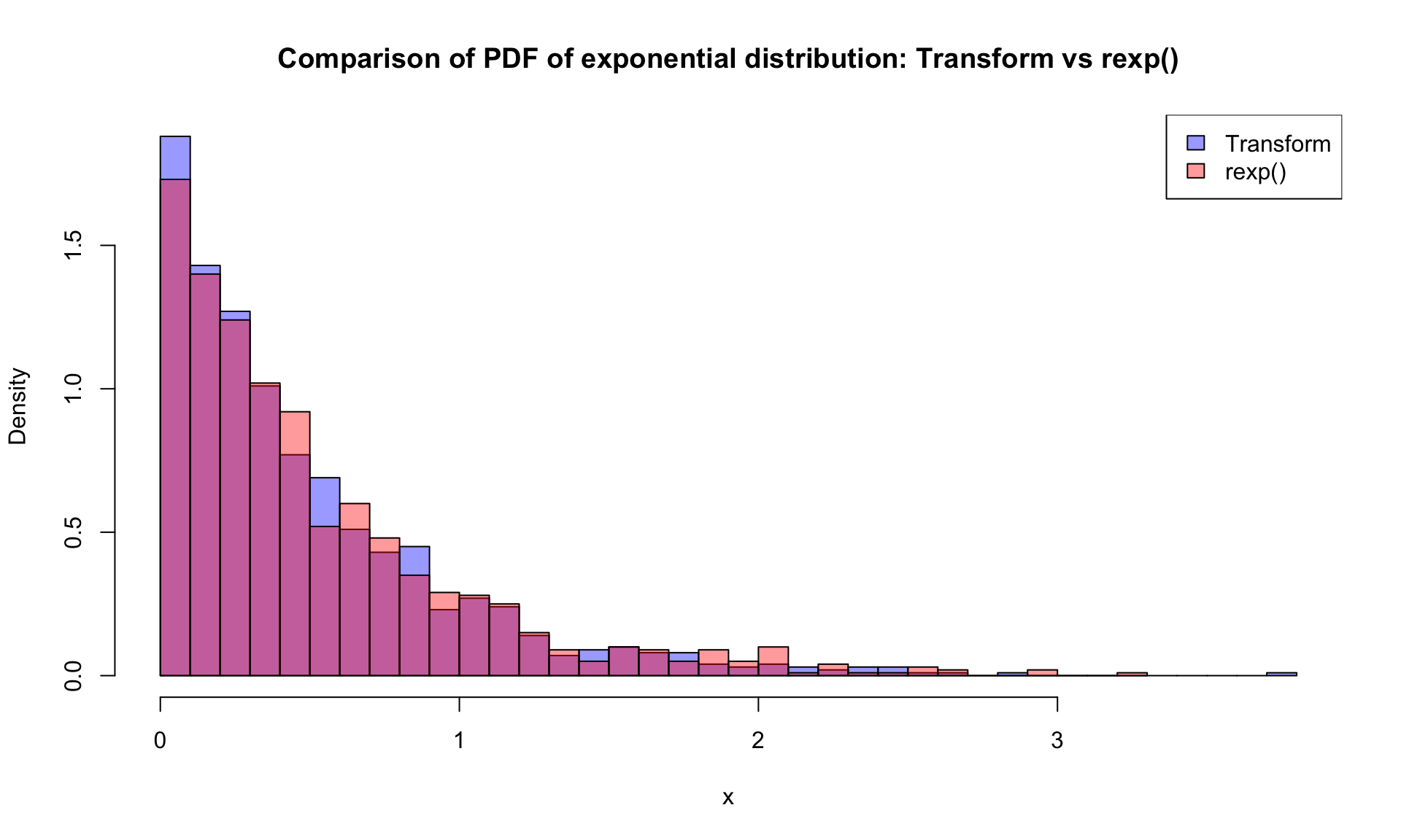
set.seed(123)
# Step 1: generate Uniform(0,1) values
u <- runif(1000)

# Step 2: transform them into Exponential(lambda)
lambda <- 2   # rate parameter
x <- -log(1 - u) / lambda

# Step 3: Plot and compare with R's built-in rexp()
x_builtin <- rexp(1000, rate = lambda)
hist(x, breaks = 30, col = rgb(0,0,1,0.4), freq = FALSE,
     main = "Comparison of PDF of exponential distribution: Transform vs rexp()")
hist(x_builtin, breaks = 30, col = rgb(1,0,0,0.4), freq = FALSE, add = TRUE)
legend("topright", legend = c("Transform", "rexp()"),
       fill = c(rgb(0,0,1,0.4), rgb(1,0,0,0.4)))
1.5 Revision: Probability Tools for Simulation

1.5.1 Basic Concepts and Definitions

Sample space (\(\Omega\)): The set of all possible outcomes of an experiment.
For example, a sample space for rolling a fair die is \(\Omega = \{1,2,3,4,5,6\}.\)

Event (\(A\)): A subset of the sample space. For example, let \(x\) be an individual’s total cholesterol in mg/dL, the event that an individual has high cholesterol is \(A = \{x\in \Omega \,|\, x > 200 \}.\) Or, for a single die roll, \(A = \{1,4,6\}.\)

Complement (\(A^c\)): The event that \(A\) does not occur. From the previous example, \(A^c = \{2,3,5\}.\)

Union (\(A \cup B\)): The event that either \(A\) occurs or \(B\) occurs. Let \(A=\{1,2\}\) and \(B= \{1, 3, 5\}\). Then \(A \cup B = \{1, 2, 3, 5 \}.\)

Intersection (\(A \cap B\)): The event that both \(A\) and \(B\) occur. Using the previous example, \(A \cap B = \{1\}\).

Disjoint: Events that have no outcomes in common. For example, if \(A=\{2, 4, 6 \}\) and \(B= \{1, 3, 5\}\), then \(A\) and \(B\) are disjoint since \(A \cap B = \emptyset\), where \(\emptyset\) represents the empty set (the set with no elements).

1.5.1 Basic Concepts and Definitions (continue)

We have the following laws for any three events \(A, B, C \subseteq \Omega.\)

  • Commutative Laws: \[ \begin{align*} A \cup B &= B \cup A \\ A \cap B &= B \cap A \end{align*} \]

  • Associative Laws: \[ \begin{align*} A \cup (B \cup C) &= (A \cup B) \cup C \\ A \cap (B \cap C) &= (A \cap B) \cap C \end{align*} \]

  • Distributive Laws: \[ \begin{align*} A \cap (B \cup C) &= (A \cap B) \cup (A \cap C) \\ A \cup (B \cap C) &= (A \cup B) \cap (A \cup C) \end{align*} \]

  • De Morgan’s Laws: \[ \begin{align*} (A \cup B)^c &= A^c \cap B^c \\ (A \cap B)^c &= A^c \cup B^c \end{align*} \]

1.5.2 Axioms of Probability

For any random experiment, \(P\) is a probability measure defined on a sample space \(\Omega\), such that the following axioms are satisfied.

  1. \(P(\Omega) = 1\)
  2. If \(A \subseteq \Omega\) is an event, then \(P(A) \ge 0\)
  3. If \(A\) and \(B\) are disjoint, then \[ P(A \cup B) = P(A) + P(B) \] This axiom extends to any finite (or countable) collection of pairwise disjoint events.

Properties of Probability Measures

  1. \(P(A^c) = 1 - P(A)\)
  2. \(P(\emptyset) = 0\)
  3. If \(A \subseteq B\), then \(P(A) \le P(B)\)

Addition Law: \[P(A \cup B) = P(A) + P(B) - P(A \cap B)\]

1.5.3 Law of Total Probability

Let \(A_i\) for \(i=1,\ldots, k\) be mutually exclusive and exhaustive events, i.e. \(\displaystyle \cup^k_{i=1} A_i = \Omega\), and \(B\) be any other event. \[ P(B) = P\left [ B \cap \left ( \overset{k}{\underset{i=1}{\cup}} A_i \right ) \right ] = \sum^k_{i=1} P(B \cap A_i ) = \sum^k_{i=1} P(B|A_i)P(A_i) \]

1.5.4 Conditional Probability

For any events \(A\) and \(B,\) conditional probability is defined as: \[ P(A|B) = \frac{P(A \cap B)}{P(B)} \quad \text{ provided that } \quad P(B) \ne 0 \]

Rearranging the conditional probability formula gives the Multiplication Rule for probabilities: \[P(A \cap B) = P(A|B) P(B) = P(B|A) P(A)\]

If the probability of \(A\) is not affected by whether or not event \(B\) occurs, then \(A\) is said to be independent of \(B\). \[ P(A|B) = P(A) \quad \text{ and } \quad P(B) \neq 0 \quad \Leftrightarrow \quad P(A \cap B)=P(A)P(B)\]

1.5.5 Bayes’ Theorem

For mutually exclusive and exhaustive events, \(B_1, B_2, \ldots, B_n, P(B_k|A) = \dfrac{P(A|B_k) P(B_k)}{\sum_{i=1}^n P(A|B_i)P(B_i)}\)

1.5.6 Random Variables

A random variable (RV) is a numerical quantity whose value is determined by a random process.

  • It’s a mapping from outcomes → numbers
  • It’s how probability becomes something we can compute with
  • It’s the bridge between randomness and simulation

In simulation, random variables are the objects we generate.

Everything they do later is built on the ability to generate RVs with specific distributions. In other word,

RVs are the currency of simulation.

DISCRETE

Take countable values

Examples

  • Number of customers arriving in an hour
  • Number of heads in 10 flips
  • Poisson, Binomial, Geometric
CONTINUOUS

Take values in an interval

Examples

  • Waiting time
  • Service duration
  • Normal, Exponential, Uniform

PMF/PDF

CDF

E(X) & Var(X)

1.5.7 Probability Distributions (PMF / PDF / CDF)

  • The distribution of probabilities for a discrete RV can be described by its probability mass function (PMF), \[p(x) = P(X=x).\]

  • The distribution of probabilities for a continuous RV can be described by its probability density function (PDF), \[f(x) \geq 0 \quad \forall x, \quad \int^\infty_{-\infty} f(x)\,dx = 1 \quad \text{ and } \quad P(a\leq X \leq b) = \int_a^b f(x)\,dx.\]

  • The cumulative distribution function (CDF) for the RV \(X\) is \(F(x) = P ( X\leq x)\) (discrete & continuous) \[F(x)= \int_{-\infty}^x f(t)\,dt. \quad \text{(continuous)}\]

1.5.8 Expectation \(E(X)\) or \(\mu\)

  • Let \(X\) be a discrete RV with a set of possible values \(D\), then \(\displaystyle \mathbb{E} (X) = \underset{x\in D}{\sum} xp(x)\)

  • Let \(X\) be a continuous RV with the support \(D\), then \(\displaystyle \mathbb{E} (X) = \int_D xf(x) \,dx\)

Properties of the Expectation Operator

  • Constant rule: If \(a\) is a finite constant, then \(\mathbb{E} (a) = a.\)

  • Linearity of expectation: For any RVs \(X\), \(Y\), and any constants \(a,b \in \mathbb{R},\) \[\mathbb{E} (aX + bY)=a\mathbb{E} (X) + b \mathbb{E} (Y).\]

  • Expectation of a function: For any function \(h(x)\) such that the expectation exists,

    • if \(X\) is a discrete RV with a set of possible values \(D\) and PMF \(p(x),\) then \[ \mathbb{E} \left [ h(X) \right ] = \underset{x\in D}{\sum} h(x)p(x) \quad\text{provided the sum converges.}\]

    • if \(X\) is a continuous RV with support \(D\) and PDF \(f(x),\) then \[ \mathbb{E} \left [ h(X) \right ] = \int_D h(x)f(x)\,dx \quad \text{provided the integral exists.}\]

1.5.9 Variance \(Var(X)\) or \(\sigma^2\)

Let \(h(x) = \left (x-\mathbb{E} [X] \right )^2,\) then \(Var(X) = \mathbb{E} \left [ h(x) \right ] = \mathbb{E} [(x-\mathbb{E}[X])^2] = \mathbb{E}[X^2] - \mathbb{E}[X]^2.\)

The variance is also known as the second centralised moment. \(\sigma_X\) is the standard deviation of \(X.\)

Higher order moment: Let \(h(x) = \left [ X-\mathbb{E} (X) \right ]^n\), then \(\mathbb{E} [h(x)]\) is called the \(n^{th}\) centralised moment (if exists). These are associated with other properties of the probability distributions, e.g., skewness and kurtosis.

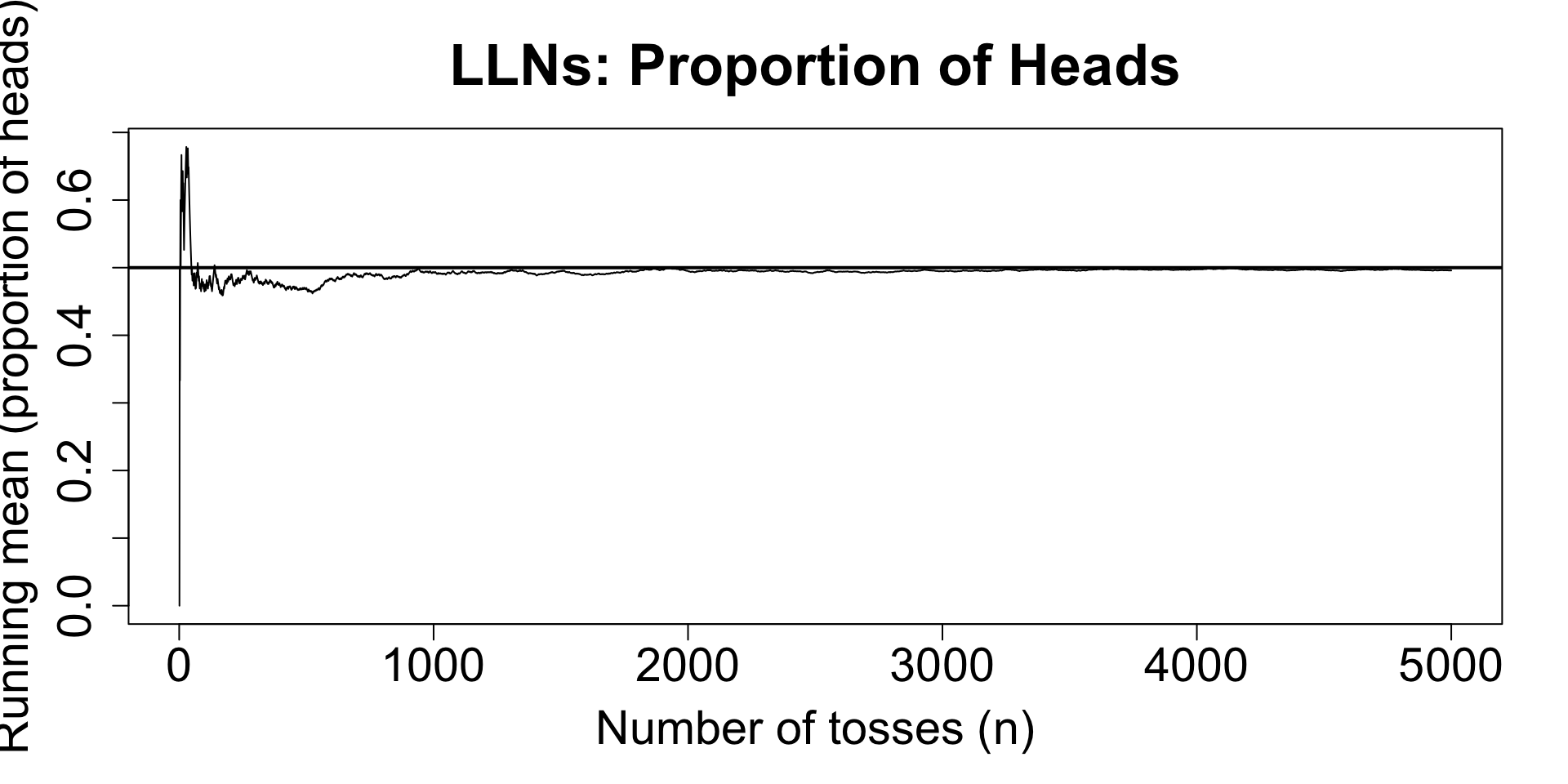
1.5.10 Law of Large Numbers (LLNs)

If we repeat the same random experiment many times, the average result stabilises.

Let \(X_1, X_2, \dots, X_n\) be independent, identically distributed (i.i.d.) with mean \(E[X]\).

Then as \(n \to \infty,\) \[ \bar{X}_n=\frac{1}{n}\sum_{i=1}^n X_i \;\longrightarrow\; E[X] \] (in the sense that the average gets closer to the true mean).

Simulation takeaway: more replications \(n \Rightarrow\) more stable estimates (but never perfectly exact).

Flipping a fair coin for 5000 times.
# Demonstrate the LLN with coin tosses
x <- rbinom(5000, size = 1, prob = 0.5)   # 1 = Head, 0 = Tail
running_mean <- cumsum(x) / seq_len(n)

plot(running_mean, type = "l",
     xlab = "Number of tosses (n)",
     ylab = "Running mean (proportion of heads)",
     main = "LLNs: Proportion of Heads",
     cex.main = 2.2,
     cex.lab = 1.8,
     cex.axis = 1.8,
     )

abline(h = 0.5, lwd = 2)  # true mean
Simulate Exp(1) for 5000 times.
# LLN with an Exponential(1) random variable (true mean = 1)
x <- rexp(n, rate = 1)
running_mean <- cumsum(x) / seq_len(n)

plot(running_mean, type = "l",
     xlab = "Number of samples (n)",
     ylab = "Running mean",
     main = "LLNs: Exponential(1)",
      cex.main = 2.2,
     cex.lab = 1.8,
     cex.axis = 1.8,
     )

abline(h = 1, lwd = 2)  # true mean