STAT2005 Computer Simulation

Lecture 2 — Statistical Distributions

Sam Wiwatanapataphee (275287a@curtin.edu.au)

26 Feb 2026

Goals today

  • Part 1: Univariate distributions in simulation
    • Discrete distributions
      • Bernoulli
      • Binomial
      • Geometric
      • Negative Binomial
      • Poisson
      • Multinomial
    • Continuous distributions
      • Uniform
      • Exponential
      • Gamma
      • Normal
      • Log-Normal
      • Beta
  • Part 2: Joint distributions and dependence
    • Joint distributions
    • Independence
    • Conditional distribution
    • Covariance and correlation
    • Bivariate normal distribution

If deep learning can predict outcomes from data, why do we still need statistical simulation?

Deep learning is powerful
if historical data fully represents the future.

but in reality, that assumption fails… our data will never be perfect!

Deep learning predicts what is likely (given the data).
Simulation explores what is possible (under uncertainty and risk).

When the future may differ from the past,
managing uncertainty beats accuracy.

Risk management matters more than point prediction.

Part 1: Univariate distributions in simulation

The vibe for Part 1…

You already know (most of) the formulas.

Today is about modelling choices.

  • What kind of randomness is in your system?
  • What does the random variable represent?
  • Which distribution is a reasonable model?

A modelling-first question

When you simulate a system, what are you modelling?

  • Counts (how many?)
  • Wait times / durations (how long?)
  • Binary events (yes/no?)
  • Category choices (which one?)
  • Uncertain probabilities (how sure are we about p?)

One slide cheat-sheet


Simulation question Typical distribution
Is it yes/no? (binary) Bernoulli
# successes in n trials Binomial
# trials until first success Geometric
# trials until r successes Negative Binomial
# arrivals in time window Poisson
Which category (K options)? Multinomial
Value equally likely in range Uniform
Time until next event Exponential
Sum of waiting times / flexible duration Gamma
Many small effects add up Normal
Multiplicative growth Log-normal
Random probability in (0,1) Beta

R Functions for Probability Distributions

The naming structure follows the pattern prefix + distribution, where the prefix:

  • d — density or mass function
  • p — cumulative distribution function
  • q — quantile function (inverse CDF)
  • r — random number generation
Distribution PDF / PMF CDF Quantile Random Generation
Binomial dbinom(x, size, prob) pbinom() qbinom() rbinom()
Geometric dgeom(x, prob) pgeom() qgeom() rgeom()
Negative Binomial dnbinom(x, size, prob, mu) pnbinom() qnbinom() rnbnom()
Poisson dpois(x, lambda) ppois() qpois() rpois()
Multinomial dmultinom(x, size, prob) - - rmultinom()
Exponential dexp() pexp() qexp() rexp()
Uniform dunif(x, min, max) punif() qunif() runif()
Exponential dexp(x, rate) pexp() qexp() rexp()
Gamma dgamma() pgamma() qgamma() rgamma()
Normal dnorm(x, mean, sd) pnorm() qnorm() rnorm()
Log-normal dlnorm(x, meanlog, sdlog) plnorm() qlnorm() rlnorm()
Beta dbeta(x, shape1, shape2) pbeta() qbeta() rbeta()
t dt(x, df) pt() qt() rt()
Chi-square dchisq(x, df) pchisq() qchisq() rchisq()

A single running example: coffee shop


We’ll reuse this throughout the lecture.


  • Customers arrive randomly
  • Service times vary
  • Some customers leave (abandon)
  • Customers choose different drink categories
  • Daily demand changes with randomness

We will simulate it, not solve it by formulas.

Discrete distributions

Discrete = counts, trials, categories

PMF: \(\displaystyle p(x) = P(X = x)\)

Conditions: \(\displaystyle p(x) \ge 0 \;\; \forall x, \quad \sum_x p(x) = 1.\)

CDF: \(\displaystyle F(x) = P(X \le x) = \sum_{t \le x} p(t).\)


We can categorise discrete distributions into:

  1. Single-Trial Model
    • Bernoulli → binary events, indicators, acceptance decisions
  2. Repeated Independent Trials
    • Binomial → total successes across repetitions
    • Geometric → time to first event (waiting time)
    • Negative Binomial → flexible count modelling
  3. Count Processes
    • Poisson → event counts in time/space
  4. Multi-Category Outcomes
    • Multinomial → categorical sampling, Markov transitions

X ~ Bernoulli(p): a binary switch

Why it matters in simulation:

It is an atomic unit of discrete randomness that is used to constructed many complex models. It underlies:

  • Acceptance–rejection algorithms (accept = 1, reject = 0)
  • Indicator variables in Monte Carlo estimation
PMF \(P(X=x) = p^x(1-p)^{1-x} \quad \text{for } x \in \{0,1\}.\) E(X) \(\mathbb{E}[X]=p\)
CDF \(F(x) = \begin{cases} 0 & x<0, \\ 1-p & 0 \leq x \lt 1, \\ 1 & x \geq 1. \end{cases}\) Var(X) \(\mathrm{Var}(X)=p(1-p)=pq.\)
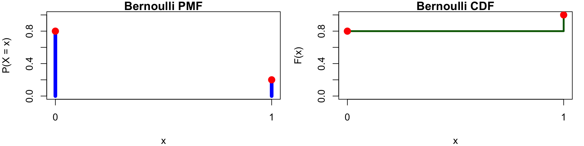
Bernoulli(0.2) PMF and CDF
# Parameter
p <- 0.2   # Probability of success

# Possible values
x <- c(0, 1)

# PMF and CDF
pmf <- dbinom(x, size = 1, prob = p)
cdf <- pbinom(x, size = 1, prob = p)

# Set plotting area to 1 row, 2 columns
par(mfrow = c(1, 2), mar = c(4, 4, 1, 1))

# --- PMF Plot ---
plot(x, pmf,
     type = "h",
     lwd = 6,
     col = "blue",
     ylim = c(0, 1),
     xaxt = "n",
     main = "Bernoulli PMF",
     xlab = "x",
     ylab = "P(X = x)")

axis(1, at = x) # manually adds tick marks
points(x, pmf, pch = 19, col = "red", cex = 1.5)

# --- CDF Plot ---
plot(x, cdf,
     type = "s",
     lwd = 3,
     col = "darkgreen",
     ylim = c(0, 1),
     xaxt = "n",
     main = "Bernoulli CDF",
     xlab = "x",
     ylab = "F(x)")

axis(1, at = x) # manually adds tick marks
points(x, cdf, pch = 19, col = "red", cex = 1.5)

Examples - customer abandons queue (yes/no) - machine fails today (yes/no) - email is spam (yes/no)

set.seed(1)
x <- rbinom(20, size = 1, prob = 0.2)
x
 [1] 0 0 0 1 0 1 1 0 0 0 0 0 0 0 0 0 0 1 0 0
mean(x)  # simulated rate
[1] 0.2
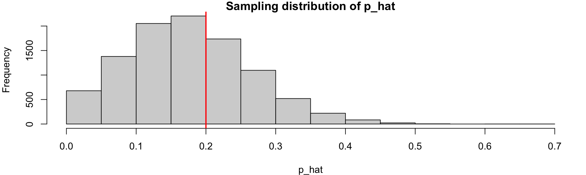
B <- 10000; n <- 20; p <- 0.2
p_hats <- replicate(B, mean(rbinom(n, 1, p))) # simulate many times

par(mar = c(4, 4, 1, 1))
hist(p_hats, breaks = 20, main = "Sampling distribution of p_hat", xlab = "p_hat")
abline(v = p, col = "red", lwd = 2)

X ~ Binomial(n,p): number of successes in n trials

Why it matters in simulation: Binomial counts often measure performance metrics across repeated trials.

  • Models aggregated binary outcomes.
  • Appears in reliability systems (number of working components).
  • Used in bootstrap and resampling procedures.
  • Forms a bridge between Bernoulli and Poisson processes.
PMF \(P(X=k)=\binom{n}{k}p^k(1-p)^{n-k}\) E(X) \(\mathbb{E}[X]=np\)
CDF \(\sum_{k=0}^x P(X=k)\) Var(X) \(\mathrm{Var}(X)=np(1-p)\)
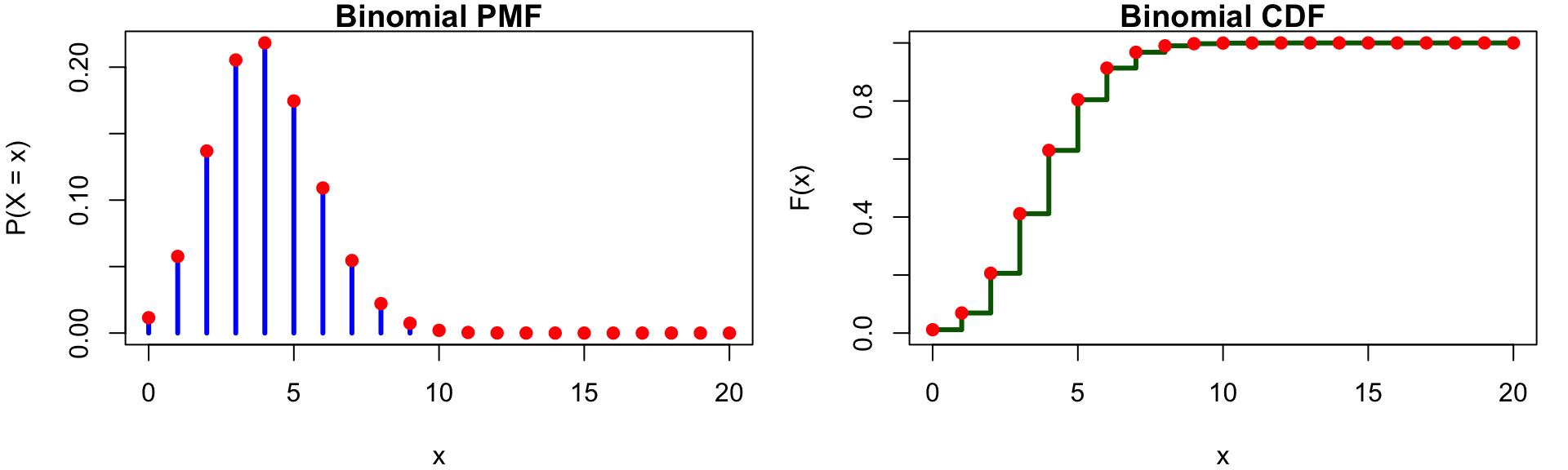
Binomial(20, 0.2) PMF and CDF
# Parameters
n <- 20      # number of trials
p <- 0.2     # probability of success

# Possible values
x <- 0:n

# PMF and CDF
pmf <- dbinom(x, size = n, prob = p)
cdf <- pbinom(x, size = n, prob = p)

# Set plotting area: 1 row, 2 columns
par(mfrow = c(1, 2), mar = c(4, 4, 1, 1))

# --- PMF Plot ---
plot(x, pmf,
     type = "h",
     lwd = 3,
     col = "blue",
     main = "Binomial PMF",
     xlab = "x",
     ylab = "P(X = x)",
     ylim = c(0, max(pmf)))

points(x, pmf, pch = 19, col = "red")

# --- CDF Plot ---
plot(x, cdf,
     type = "s",
     lwd = 3,
     col = "darkgreen",
     main = "Binomial CDF",
     xlab = "x",
     ylab = "F(x)",
     ylim = c(0, 1))

points(x, cdf, pch = 19, col = "red")

Examples - defective items in a batch of n - latte art done perfectly out of n attempts

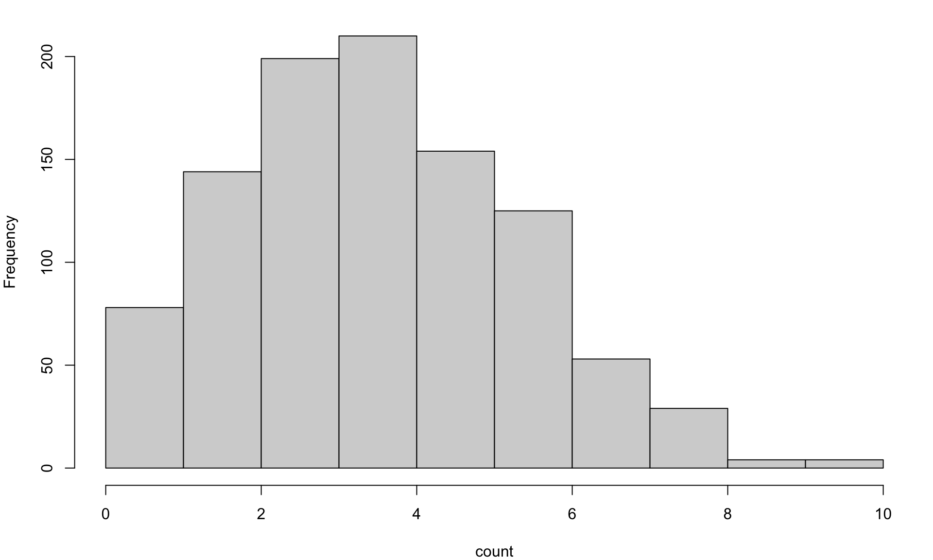
set.seed(2)
y <- rbinom(1000, size = 20, prob = 0.2)
par(mar = c(4, 4, 1, 1))
hist(y, main="", xlab = "count")

X ~ Geometric(p): trials until first success

Why it matters in simulation:

  • Represents waiting times in discrete-time systems.
  • Discrete analogue of the exponential distribution.
  • Possesses the memoryless property, making it important in stochastic process theory.
  • Useful in modelling repeated attempts (e.g., retry mechanisms in networks).
PMF \(P(X = k) = (1 - p)^{k - 1} p, \quad k\in \mathbb{N}={1,2,3,...}\) E(X) \(E[X] = 1/p\)
CDF \(P(X \leq k) = 1 - (1 - p)^k\) Var(X) \(\text{Var}[X] = (1 - p)/p^2\)
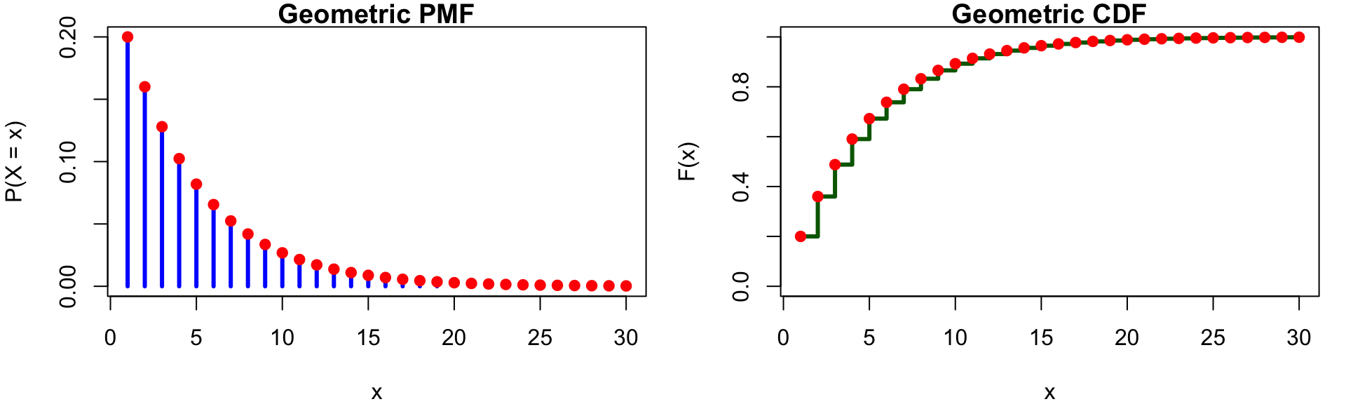
Geometic(0.2) PMF and CDF
# Parameters
n <- 30      # number of trials
p <- 0.2     # probability of success

# Possible values
x <- 1:n

# PMF and CDF
pmf <- dgeom(x-1, prob = p)
cdf <- pgeom(x-1, prob = p)

# Set plotting area: 1 row, 2 columns
par(mfrow = c(1, 2), mar = c(4, 4, 1, 1))

# --- PMF Plot ---
plot(x, pmf,
     type = "h",
     lwd = 3,
     col = "blue",
     main = "Geometric PMF",
     xlab = "x",
     ylab = "P(X = x)",
     ylim = c(0, max(pmf)))

points(x, pmf, pch = 19, col = "red")

# --- CDF Plot ---
plot(x, cdf,
     type = "s",
     lwd = 3,
     col = "darkgreen",
     main = "Geometric CDF",
     xlab = "x",
     ylab = "F(x)",
     ylim = c(0, 1))

points(x, cdf, pch = 19, col = "red")

Examples - defective items in a batch of n - latte art done perfectly out of n attempts

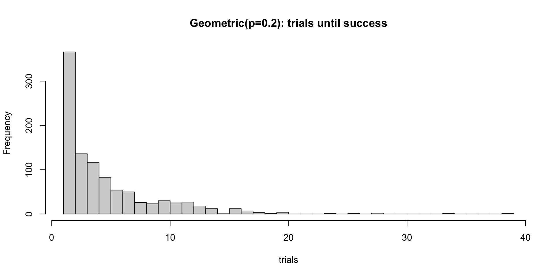
set.seed(3)
g <- rgeom(1000, prob = 0.2) + 1  # R's rgeom returns failures before first success
mean(g)
[1] 4.876
hist(g, breaks = 30, main = "Geometric(p=0.2): trials until success", xlab = "trials")

X ~ NegativeBinomial(r, p): trials until r success

Why it matters in simulation:

  • Models overdispersed count data (variance greater than mean).
  • Frequently used in arrival modelling when Poisson assumptions are too restrictive.
  • Arises as a mixture of Poisson distributions (important in Bayesian modelling).
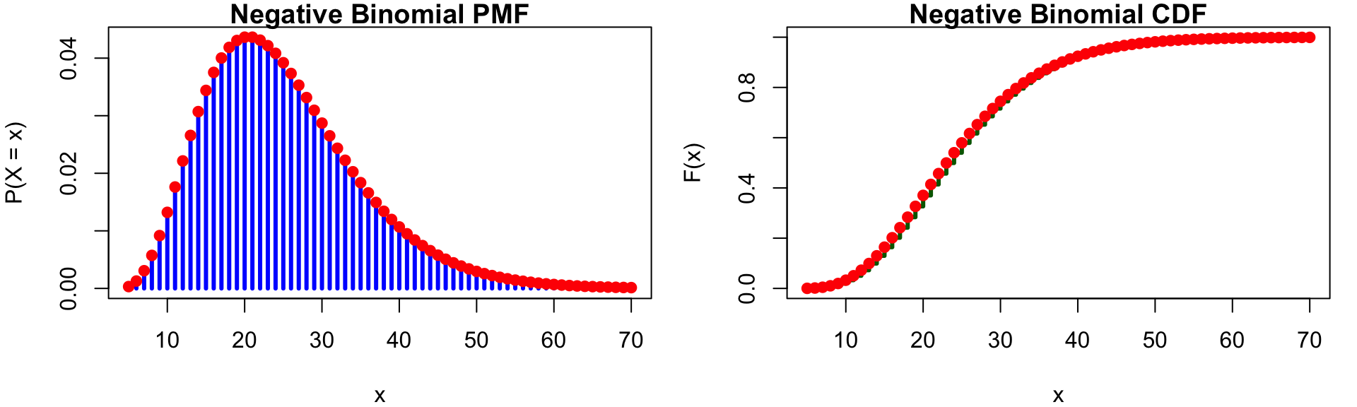
PMF \(P(X = r) = \binom{x - 1}{r-1} p^r (1 - p)^{x-r}\) E(X) \(E[X] = r/p\)
CDF \(P(X \leq k) = \displaystyle\sum_{k=0}^x P(X=k)\) Var(X) \(\text{Var}[X] = \dfrac{r(1 - p)}{p^2}\)
NegBin(2,0.2) PMF and CDF
# Parameters
max_x <- 70  # number of trials
r <- 5       # number of successes
p <- 0.2     # probability of success

# Possible values
x <- r:max_x

# PMF and CDF
pmf <- dnbinom(x-r, size = r, prob = p)
cdf <- pnbinom(x-r, size = r, prob = p)

# Set plotting area: 1 row, 2 columns
par(mfrow = c(1, 2), mar = c(4, 4, 1, 1))

# --- PMF Plot ---
plot(x, pmf,
     type = "h",
     lwd = 3,
     col = "blue",
     main = "Negative Binomial PMF",
     xlab = "x",
     ylab = "P(X = x)",
     ylim = c(0, max(pmf)))

points(x, pmf, pch = 19, col = "red")

# --- CDF Plot ---
plot(x, cdf,
     type = "s",
     lwd = 3,
     col = "darkgreen",
     main = "Negative Binomial CDF",
     xlab = "x",
     ylab = "F(x)",
     ylim = c(0, 1))

points(x, cdf, pch = 19, col = "red")

Examples - calls until 5 sales - customers until 10 purchases - experiments until r “good” outcomes

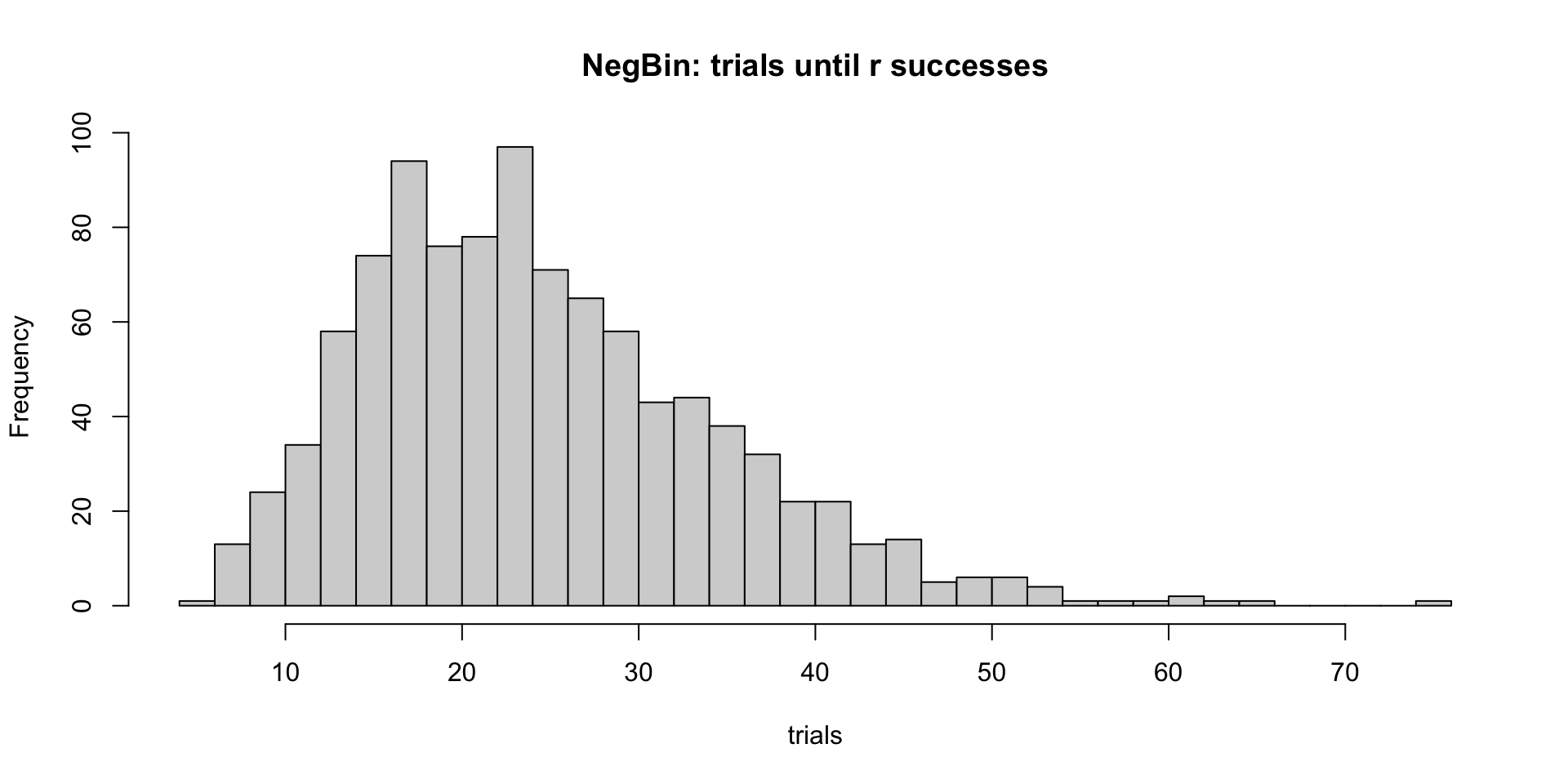
set.seed(4)
r <- 5
nb <- rnbinom(1000, size = r, prob = 0.2)  # failures before r successes
trials <- nb + r
mean(trials)
[1] 24.947
hist(trials, breaks = 30, main = "NegBin: trials until r successes", xlab = "trials")

X ~ Poisson(\(\lambda\)): counts in a time window

Why it matters in simulation:

  • Fundamental to queueing theory.
  • Governs random arrival systems.
  • Provides a natural approximation to binomial counts with rare events.
  • Plays a central role in discrete-event simulation.
PMF \(P(X=k)=\dfrac{e^{-\lambda}\lambda^k}{k!}\) E(X) \(E[X] = \lambda\)
CDF \(\displaystyle P(X \leq k) = e^{\lambda}\sum_{j=0}^{\lfloor k \rfloor}\dfrac{\lambda^j}{j!}\) Var(X) \(\text{Var}[X] = \lambda\)
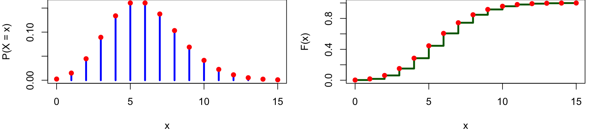
Poisson(6) PMF and CDF
# Parameters
lambda <- 6   # mean (rate)

# Reasonable range of x values
x <- 0:(lambda + 4*sqrt(lambda))
x <- 0:max(x)

# PMF and CDF
pmf <- dpois(x, lambda = lambda)
cdf <- ppois(x, lambda = lambda)

# Set plotting area: 1 row, 2 columns
par(mfrow = c(1, 2), mar = c(4, 4, 0, 1))

# --- PMF Plot ---
plot(x, pmf,
     type = "h",
     lwd = 3,
     col = "blue",
     xlab = "x",
     ylab = "P(X = x)",
     ylim = c(0, max(pmf)))

points(x, pmf, pch = 19, col = "red")

# --- CDF Plot ---
plot(x, cdf,
     type = "s",
     lwd = 3,
     col = "darkgreen",
     xlab = "x",
     ylab = "F(x)",
     ylim = c(0, 1))

points(x, cdf, pch = 19, col = "red")

Examples - customer arrivals per hour - number of claims per day - number of defects per shift

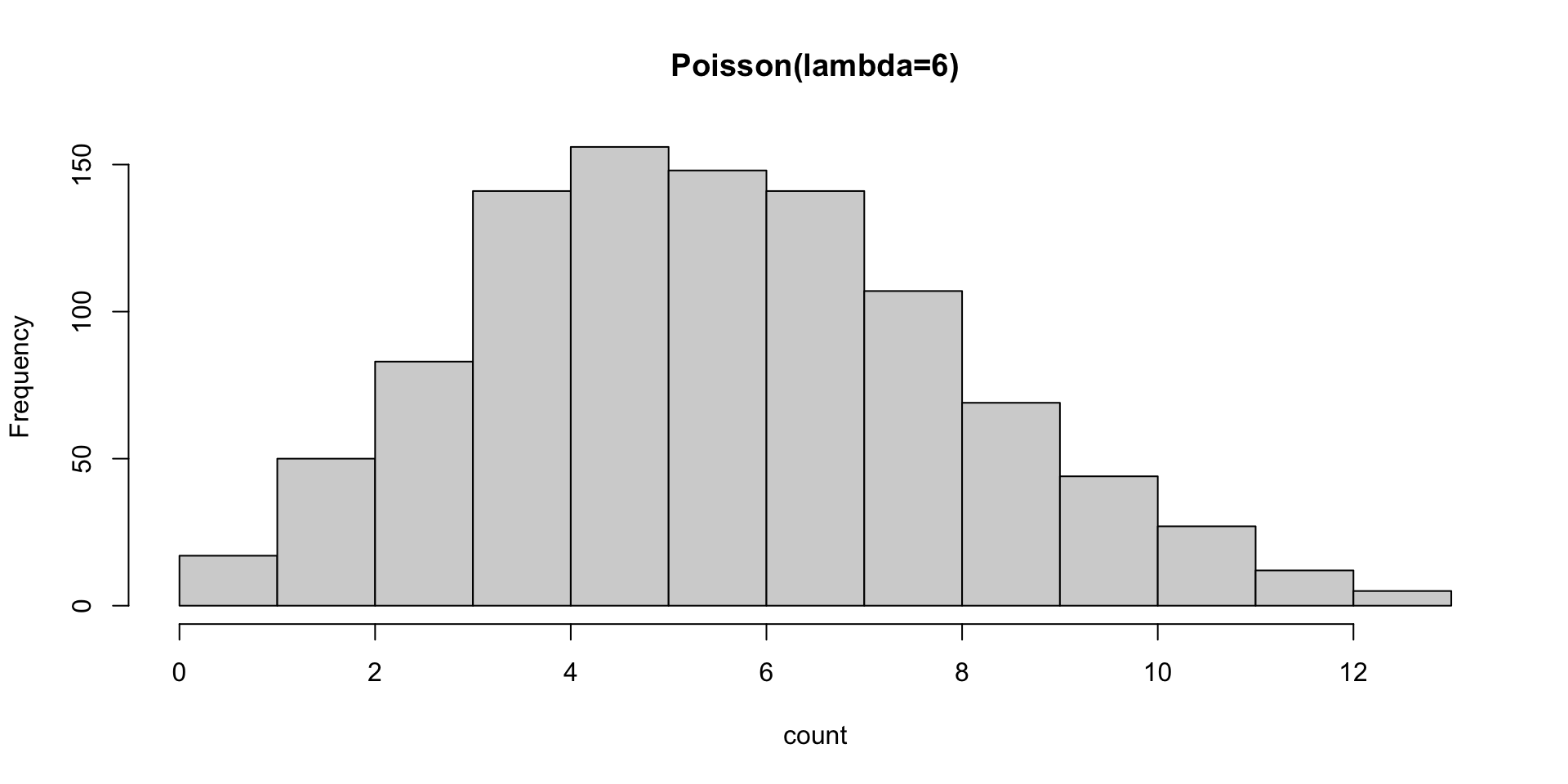
set.seed(5)
p <- rpois(1000, lambda = 6)
mean(p); var(p)
[1] 6.004
[1] 5.987972
hist(p, breaks = 10, main = "Poisson(lambda=6)", xlab = "count")

\((X_1, \dots, X_k) \sim \text{Multinomial}(n; p_1, \dots, p_k)\)


The Multinomial distribution generalises the binomial to more than two outcome categories.

Why it matters in simulation:

  • Models categorical random outcomes.
  • Essential for simulating:
    • Markov chains
    • Discrete-state stochastic processes
    • Classification and allocation models
  • Underlies Gibbs sampling in discrete settings.

In simulation algorithms, sampling from a categorical distribution is a core primitive operation.


Suppose we perform \(n\) independent trials.

Each trial results in exactly one of \(k\) possible categories, with probabilities

\[p_1, p_2, \dots, p_k, \qquad \text{where } p_i \ge 0, \quad \sum_{i=1}^k p_i = 1.\]

When \(k = 2\), the multinomial reduces to the binomial distribution.

Joint PMF \(P(X_1 = x_1, \dots, X_k = x_k) = \dfrac{n!}{x_1! x_2! \cdots x_k!} \prod_{i=1}^k p_i^{x_i}, \quad \sum_{i=1}^k X_i=n.\)
Joint CDF \(F(x_1, \dots, x_k) = P(X_1 \le x_1, \dots, X_k \le x_k).\)
E(X) \(E[X] = np_i\)
Var(X) \(\text{Var}[X] = np_i(1-p_i)\)


Note: The multinomial’s mean and variance resemble the binomial’s mean and variance because each \(X_i\) marginally follows \(X_i \sim \text{Binomial}(n,p_i)\)

Example: Imagine a busy coffee shop during the morning rush. Ten customers \((n = 10)\) arrive one after another, and each customer randomly chooses one of six drink types, all equally likely: Espresso, Latte, Cappuccino, Mocha, Flat White, and Long Black. Assume each drink is chosen with probability 1/6. Then,

\[ (X_1, X_2, X_3, X_4, X_5, X_6) \sim \text{Multinomial}\left(10; \frac16, \frac16, \frac16, \frac16, \frac16, \frac16\right). \]

Now suppose that after serving 10 customers, the barista looks at the tally sheet and sees:

  • 2 Espressos
  • 1 Latte
  • 3 Cappuccinos
  • 0 Mochas
  • 2 Flat Whites
  • 2 Long Blacks

This corresponds exactly to \((x_1,x_2,x_3,x_4,x_5,x_6) = (2,1,3,0,2,2)\).

The probability of \((x_1,x_2,x_3,x_4,x_5,x_6) = (2,1,3,0,2,2)\) is \(\dfrac{10!}{2!1!3!0!2!2!}\left(\dfrac{1}{6}\right)^{10} = 0.00125\)

dmultinom(x = c(2,1,3,0,2,2), prob = rep(1/6, 6))
[1] 0.001250286

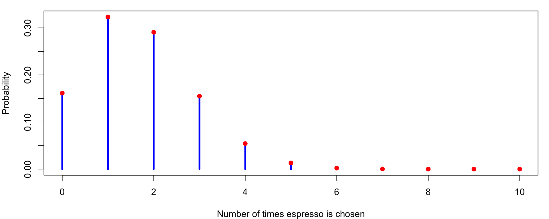
The multinomial distribution is multivariate, so it does not have a simple 1D PMF curve.

Instead, we can visualise a marginal distribution of one drink type, which is \(X_i \sim \text{Binomial}(10,1/6)\).

Marginal Distribution of \(X_1\)
n <- 10
p <- 1/6
k <- 0:n
pmf <- dbinom(k, size = n, prob = p)
par(mar = c(4, 4, 1, 1))
plot(k, pmf,
     type = "h",
     lwd = 3,
     col = "blue",
     xlab = "Number of times espresso is chosen",
     ylab = "Probability",
     ylim = c(0, max(pmf)))
points(k, pmf, pch = 19, col = "red")

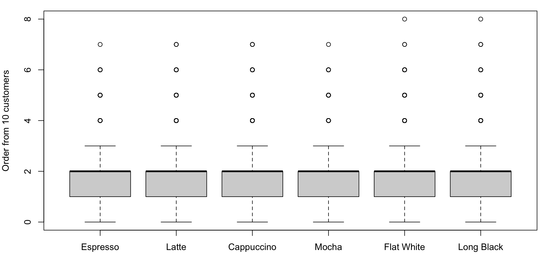
Instead, we can try simulating many multinomial experiments and visualise the counts.

Simulated Multinomial Counts
set.seed(123)
sim <- rmultinom(10000, size = 10, prob = rep(1/6, 6))
par(mar = c(4, 4, 1, 1))
boxplot(t(sim),
        names = c("Espresso", "Latte", "Cappuccino", "Mocha", "Flat White", "Long Black"),
        ylab = "Order from 10 customers")
  • All six boxplots look almost identical because each face has the same marginal distribution and probability.
  • The counts fluctuate around about 1 or 2, which matches the expected value of 10 divided by 6.
  • Notice that large order numbers (>3) are rare, since this is just 10 customers.
  • Although the boxplots look independent, the total number of orders is fixed at 10, so if one drink is ordered more often, others must appear less often.

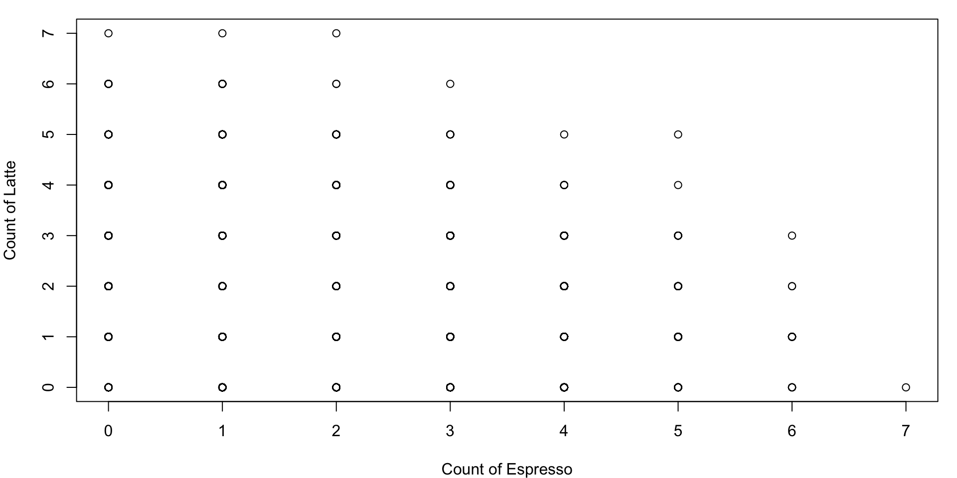
Consider the dependence between the count of Espresso \(X_1\) and the dependence of Latte \(X_2\)

Negative Dependence in Multinomial
par(mar = c(4, 4, 1, 1))
plot(sim[1,], sim[2,],
     xlab = "Count of Espresso",
     ylab = "Count of Latte")
  • As the count of Espresso increases, the possible values for Latte decrease. (The categories competes.)
  • That competition produces negative dependence, which we can literally see as a downward-sloping triangular region.

Continuous distributions

Continuous = time, size, measurement

PDF: \(\displaystyle P(a \le X \le b) = \int_a^b f(x)\,dx.\)

Conditions: \(\displaystyle f(x) \ge 0, \;\; \int_{-\infty}^{\infty} f(x)\,dx = 1.\)

CDF: \(\displaystyle F(x) = \int_{-\infty}^x f(t)\,dt.\)

We can categorise continuous distributions into:

  1. Primitive distributions
    • Uniform → foundation of simulation algorithms.
  2. Event-time distributions (positive support)
    • Exponential → waiting time for first Poisson event.
    • Gamma → sum of exponentials.
  3. Limit and noise distributions
    • Normal → limit of sums (CLT).
  4. Transformation-based distributions (shape-flexible)
    • Log-normal → exponential of normal.
    • Beta → normalised gamma variables.

\(X \sim \text{Uniform}(a,b)\)

Why it matters in simulation:

  • All inverse transform methods start from Uniform(0,1).
  • Acceptance–rejection relies on uniform draws.
  • Monte Carlo integration uses uniform sampling.
  • Random number generators are designed to approximate Uniform(0,1).
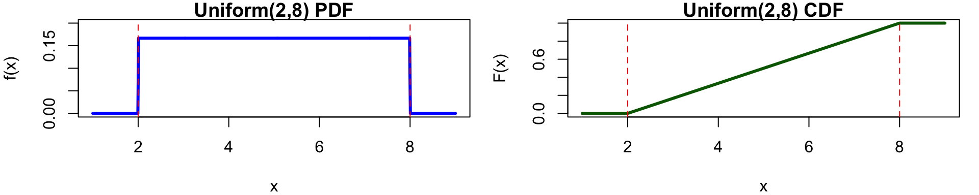
PDF \(f(x)=\dfrac{1}{b-a},\;\; a\leq x \leq b.\) E(X) \(E[X] = \dfrac{a+b}{2}\)
CDF \(F(x)=\begin{cases} 0 & x<a \\ \dfrac{x-a}{b-a} & a\leq x \leq b \\ 1 & x > b. \end{cases}\) Var(X) \(\text{Var}[X] = \dfrac{(b-a)^2}{12}\)
Uniform(2,8) PDF and CDF
# Parameters
a <- 2     # lower bound
b <- 8     # upper bound

# Sequence of x values
x <- seq(a - 1, b + 1, length = 500)

# PDF and CDF
pdf <- dunif(x, min = a, max = b)
cdf <- punif(x, min = a, max = b)

# Set plotting area: 1 row, 2 columns
par(mfrow = c(1, 2), mar = c(4, 4, 1, 1))

# --- PDF Plot ---
plot(x, pdf,
     type = "l",
     lwd = 3,
     col = "blue",
     main = paste("Uniform(", a, ",", b, ") PDF", sep=""),
     xlab = "x",
     ylab = "f(x)",
     ylim = c(0, max(pdf) * 1.2))

abline(v = c(a, b), lty = 2, col = "red")

# --- CDF Plot ---
plot(x, cdf,
     type = "l",
     lwd = 3,
     col = "darkgreen",
     main = paste("Uniform(", a, ",", b, ") CDF", sep=""),
     xlab = "x",
     ylab = "F(x)",
     ylim = c(0, 1))

abline(v = c(a, b), lty = 2, col = "red")

\(X \sim \text{Exponential}(\lambda)\)

If the number of events in any interval of length \(t\) follows \[N(t)\sim \mathrm{Poisson}(\lambda t).\]

The waiting time until the next event, \(T,\) satisfies \[P(T>t)=P(\mathrm{no\ events\ occur\ in\ }[0,t])=e^{-\lambda t}.\]

This survival function corresponds exactly to an Exponential(\(\lambda\)) distribution. Thus, \[ T\sim \mathrm{Exponential}(\lambda ). \]

So the exponential distribution is the model for inter‑arrival times in a Poisson process.

Why it matters in simulation

  • The memoryless property, \(P(X>s+t \mid X>s)=P(X>t),\) makes the distribution fundamental in
    • continuous-time Markov processes,
    • queueing theory,
    • reliability modelling (modelling system lifetime, time before failure, etc.)
  • In discrete-event simulation, inter-arrival and service times are often assumed exponential.
  • It forms the backbone of many stochastic timing models.
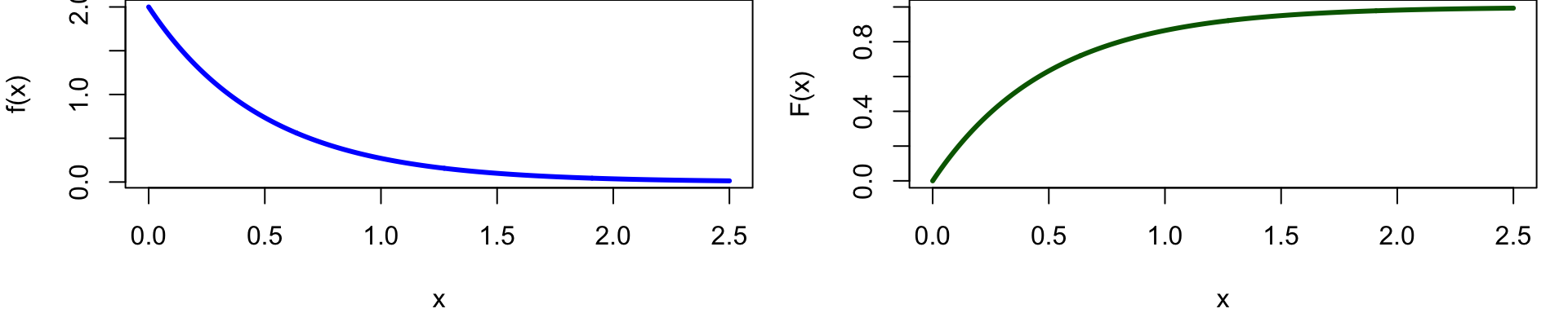
PDF \(f(x)=\lambda e^{-\lambda x}, \qquad x>0\) E(X) \(E[X] = 1/\lambda\)
CDF \(F(x)=1-e^{-\lambda x}.\) Var(X) \(\text{Var}[X] = 1/\lambda^2\)
Exponential(2) PDF and CDF
# Parameter
lambda <- 2   # rate parameter

# Sequence of x values (reasonable range)
x <- seq(0, 5/lambda, length = 500)

# PDF and CDF
pdf <- dexp(x, rate = lambda)
cdf <- pexp(x, rate = lambda)

# Set plotting area: 1 row, 2 columns
par(mfrow = c(1, 2), mar = c(4, 4, 0, 1))

# --- PDF Plot ---
plot(x, pdf,
     type = "l",
     lwd = 3,
     col = "blue",
     xlab = "x",
     ylab = "f(x)")

# --- CDF Plot ---
plot(x, cdf,
     type = "l",
     lwd = 3,
     col = "darkgreen",
     xlab = "x",
     ylab = "F(x)",
     ylim = c(0, 1))

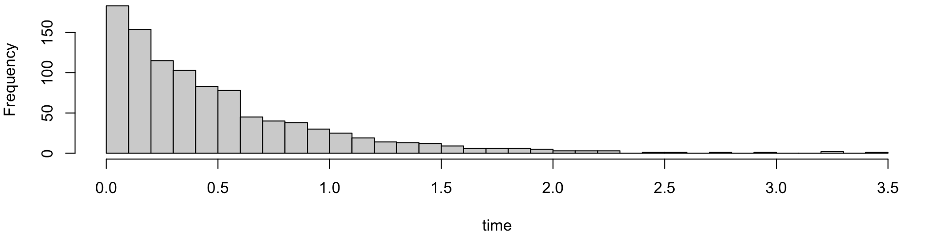
Example: - inter-arrival times (basic queueing) - time until a blending machine fails

set.seed(8); x <- rexp(1000, rate = 2); mean(x)
[1] 0.4918438
par(mar = c(4, 4, 0, 1)); hist(x, breaks = 30, main = "", xlab = "time")

Example: Linking Exponential and Poisson

Customers arrive at a coffee shop according to a Poisson process with rate \(\lambda =1.5\) customers per hour.

  • The number of arrivals in time \(t\) is \(N(t)\sim \mathrm{Poisson}(\lambda t=1.5t)\).
  • The waiting time between arrivals is \(X\sim \mathrm{Exponential}(\lambda =1.5)\).

What is the probability that the next customer arrives within 30 minutes (interarrival-time; exponential)?

\[ P(X\leq0.5)=1−e^{−1.5×0.5}=1−e^{−0.75}\approx0.528 \]

pexp(q = 0.5, rate = 1.5)
[1] 0.5276334

There is about a 52.8% chance that the next customer arrives within the next 30 minutes. This answers a waiting-time question: “How soon will the next event occur?”

What is the probability that exactly 2 customers arrive in the next hour (count; poisson)?

\[ P(N(1)=2) = \frac{e^{-1.5}1.5^2}{2!}\approx0.251 \]

dpois(x = 2, lambda = 1.5)
[1] 0.2510214

There is about a 25.1% chance that exactly two customers arrive in the next hour. This answers a count question: “How many events occur in a fixed time interval?”

\(X \sim \text{Gamma}(\alpha ,\beta)\)

Why it matters in simulation

  • Provides flexible modelling of positive, skewed data.

  • Used in reliability and survival analysis.

  • Appears as a conjugate prior in Bayesian inference.

  • Forms the basis of many hierarchical models.

It allows more realistic modelling of waiting times than the exponential, by relaxing the memoryless assumption.

PDF \(f(x)=\dfrac{\beta ^{\alpha }}{\Gamma (\alpha )}x^{\alpha -1}e^{-\beta x},\qquad x>0.\) E(X) \(E[X] = \alpha/ \beta\)
CDF \(F(x)=P(X\leq x)=\dfrac{\gamma (\alpha ,\beta x)}{\Gamma (\alpha )}\) Var(X) \(\text{Var}[X] = \alpha/ \beta^2\)
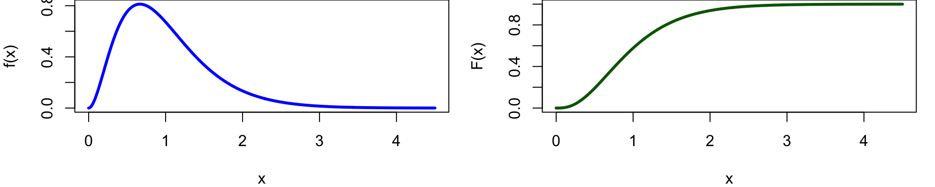
Gamma(3, 3) PDF and CDF
# Parameter
alpha <- 3   # shape parameter
beta <- 3  # rate parameter

# Sequence of x values (reasonable range)
x <- seq(0, alpha*1.5, length = 500)

# PDF and CDF
pdf <- dgamma(x, shape = alpha, rate = beta)
cdf <- pgamma(x, shape = alpha, rate = beta)

# Set plotting area: 1 row, 2 columns
par(mfrow = c(1, 2), mar = c(4, 4, 0, 1))

# --- PDF Plot ---
plot(x, pdf,
     type = "l",
     lwd = 3,
     col = "blue",
     xlab = "x",
     ylab = "f(x)")

# --- CDF Plot ---
plot(x, cdf,
     type = "l",
     lwd = 3,
     col = "darkgreen",
     xlab = "x",
     ylab = "F(x)",
     ylim = c(0, 1))

Example: The barista opens the shop at 7:00 AM. Customers arrive randomly at an average rate of 3 per minute. What is the distribution of the time until the third customer arrives?

\[ T \sim \text{Gamma}(3,3) \]

Note: As a sum of exponentials. A Gamma distribution with shape \(\alpha\) and rate \(\beta\) is the waiting time for the \(\alpha\)‑th event in a Poisson process with rate \(\beta\).

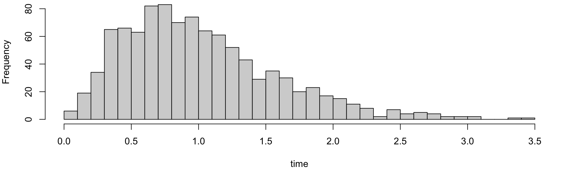
set.seed(9); z <- rgamma(1000, shape = 3, rate = 3)
mean(z)
[1] 1.01487
par(mar=c(4,4,0,1));hist(z, breaks = 30, main = "", xlab = "time")

\(X \sim \text{Normal}(\mu,\sigma^2)\)

What it matters in simulation

  • Many models assume normally distributed errors.
  • Gaussian random walks underlie MCMC algorithms.
  • Brownian motion is constructed from normal increments.
  • Variance estimation often relies on normal approximations.

Even when the true distribution is not normal, simulation output is often analysed using normal approximations.

PDF \(f(x)=\dfrac{1}{\sqrt{2\pi\sigma^2}} \exp\left(-\dfrac{(x-\mu)^2}{2\sigma^2}\right).\) E(X) \(E[X] = \mu\)
CDF \(F(x)=\Phi\left(\dfrac{x-\mu}{\sigma}\right)\) Var(X) \(\text{Var}[X] = \sigma^2\)
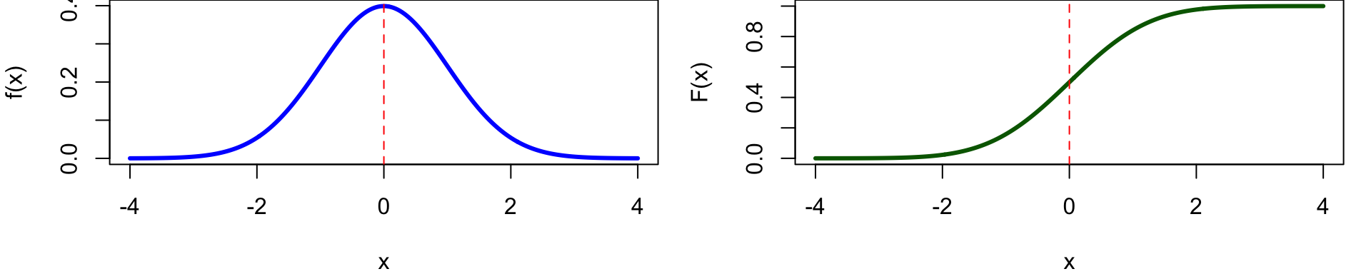
Standard Normal PMF and CDF
# Parameters
mu <- 0        # mean
sigma <- 1     # standard deviation

# Sequence of x values (cover most of the distribution)
x <- seq(mu - 4*sigma, mu + 4*sigma, length = 500)

# PDF and CDF
pdf <- dnorm(x, mean = mu, sd = sigma)
cdf <- pnorm(x, mean = mu, sd = sigma)

# Set plotting area: 1 row, 2 columns
par(mfrow = c(1, 2), mar = c(4,4,0,1))

# --- PDF Plot ---
plot(x, pdf,
     type = "l",
     lwd = 3,
     col = "blue",
     xlab = "x",
     ylab = "f(x)")

abline(v = mu, lty = 2, col = "red")

# --- CDF Plot ---
plot(x, cdf,
     type = "l",
     lwd = 3,
     col = "darkgreen",
     xlab = "x",
     ylab = "F(x)",
     ylim = c(0, 1))

abline(v = mu, lty = 2, col = "red")

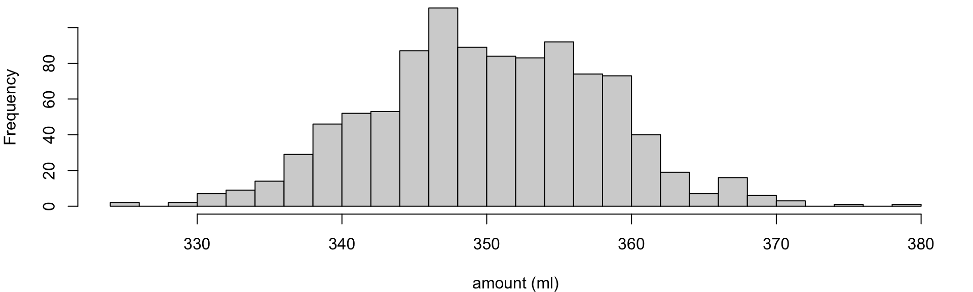
Example: Imagine a popular coffee shop that sells medium lattes. Even though the barista aims to pour exactly 350 ml each time, natural variation occurs:

  • slight differences in milk frothing
  • small timing differences when stopping the pour
  • tiny inconsistencies in cup handling

Because these small effects accumulate, the total poured volume (ml) tends to follow a Normal distribution.

\[ X \sim N(\mu=350, \sigma^2=8^2) \]

set.seed(10); z <- rnorm(1000, mean = 350, sd = 8)
par(mar=c(4,4,0,1));hist(z, breaks = 30, main = "", xlab = "amount (ml)")

\(X\sim \mathrm{Lognormal}(\mu ,\sigma ^2)\)

Why it matters in simulation

  • Used in financial modelling (asset prices).
  • Models service times with heavy right tails.
  • Arises naturally via transformation methods.
  • Demonstrates how distributions can be constructed via nonlinear transformation.
PDF \(f(x)=\dfrac{1}{x\sigma \sqrt{2\pi }}\exp \! \left( -\dfrac{(\ln x-\mu )^2}{2\sigma ^2}\right) ,\qquad x>0.\) E(X) \(E[X] = e^{\mu +\frac{1}{2}\sigma ^2}\)
CDF \(F(x)=P(X\leq x)=\Phi \! \left( \dfrac{\ln x-\mu }{\sigma }\right) ,\qquad x>0,\) Var(X) \(\text{Var}[X] = \left( e^{\sigma ^2}-1\right) e^{2\mu +\sigma ^2}\)
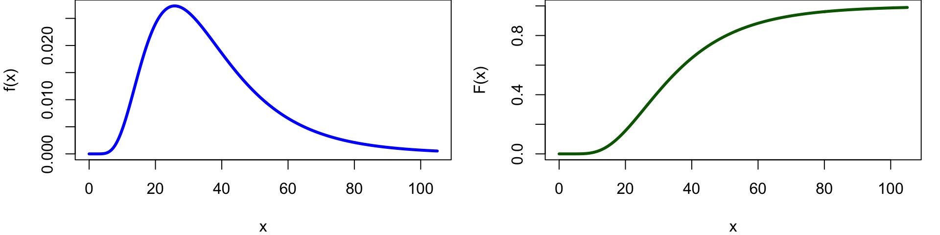
Lognormal(3.5, 0.25^2) PDF and CDF
# Parameter
mu <- 3.5   # shape parameter
sigma <- 0.5  # rate parameter

# Sequence of x values (reasonable range)
x <- seq(0, mu*30, length = 500)

# PDF and CDF
pdf <- dlnorm(x, meanlog = mu, sdlog = sigma)
cdf <- plnorm(x, meanlog = mu, sdlog = sigma)

# Set plotting area: 1 row, 2 columns
par(mfrow = c(1, 2), mar = c(4,4,0,1))

# --- PDF Plot ---
plot(x, pdf,
     type = "l",
     lwd = 3,
     col = "blue",
     xlab = "x",
     ylab = "f(x)")

# --- CDF Plot ---
plot(x, cdf,
     type = "l",
     lwd = 3,
     col = "darkgreen",
     xlab = "x",
     ylab = "F(x)",
     ylim = c(0, 1))

Example: Suppose your coffee shop sells a popular specialty drink — say, a Caramel Almond Latte. The total time to prepare one drink depends on several multiplicative factors:

  • milk‑frothing time varies by a random percentage
  • extraction time varies by a random percentage
  • syrup dispensing varies by a random percentage
  • barista speed varies by a random percentage

Each step has percentage‑based variability, not additive variability. (More realistic for human-performance tasks.)

Let T be time (in seconds) to prepare one drink. Then,

\[ \ln{T} \sim N(\mu=3.5, \sigma^2=0.5^2) \qquad\qquad T \sim \text{Lognormal}(\mu=3.5, \sigma^2=0.5^2) \]

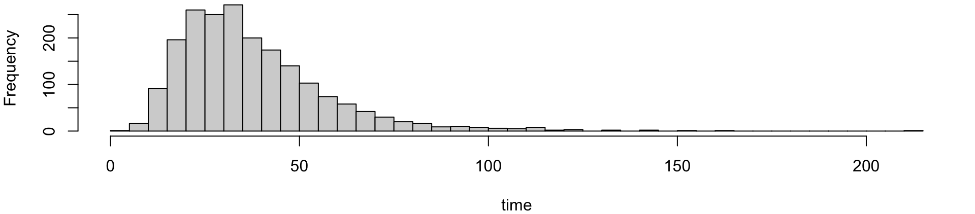
set.seed(11); ln <- rlnorm(2000, meanlog = 3.5, sdlog = 0.5)
summary(ln)
   Min. 1st Qu.  Median    Mean 3rd Qu.    Max. 
  4.803  23.724  33.253  37.525  46.102 210.575 
par(mar=c(4,4,0,1)); hist(ln, breaks = 40, main = "", xlab = "time")

\(X\sim \mathrm{Beta}(\alpha ,\beta )\)

with shape parameters \(\alpha >0\) and \(\beta >0\).

Why it matters in simulation

  • Used in Bayesian updating.
  • Models uncertainty about probabilities.
  • Appears in hierarchical simulation models.
  • Useful in sensitivity analysis.
PDF \(f(x)=\dfrac{x^{\alpha -1}(1-x)^{\beta -1}}{B(\alpha ,\beta )},\qquad 0<x<1.\) E(X) \(E[X] = \dfrac{\alpha }{\alpha +\beta }\)
CDF \(F(x)=P(X\leq x)=I_x(\alpha ,\beta )\) Var(X) \(\text{Var}[X] = \dfrac{\alpha \beta }{(\alpha +\beta )^2(\alpha +\beta +1)}\)

where the \(B(\alpha,\beta)\) is the Beta function given by

\[ B(\alpha ,\beta )=\frac{\Gamma (\alpha )\Gamma (\beta )}{\Gamma (\alpha +\beta )}, \]

and \(I_x(\alpha ,\beta )\) is the regularised incomplete beta function denoted by

\[ I_x(\alpha ,\beta ) = \frac{B(x; a,b)}{B(a,b)} \]

  • Beta distribution is highly versatile for modeling probabilities, proportions, and rates.
  • Its varied shapes — uniform, bell-shaped, U-shaped, or skewed — make it ideal for Bayesian analysis (prior/posterior), risk analysis, and modelling bounded random variables.
Beta(alpha, beta) with interactive sliders
library(plotly)
library(dplyr)
library(tidyr)

alpha_vals <- seq(.5, 5, by = .5)
beta_vals  <- seq(.5, 5, by = .5)
x_vals <- seq(0, 1, length.out = 200)

df <- expand_grid(alpha = alpha_vals,
                  beta  = beta_vals,
                  x = x_vals) %>%
  mutate(
    pdf = dbeta(x, shape1 = alpha, shape2 = beta),
    cdf = pbeta(x, shape1 = alpha, shape2 = beta),
    frame = paste0("α=", alpha, ", β=", beta)
  )

pdf_fig <- df %>%
  plot_ly(
    x = ~x, y = ~pdf,
    frame = ~frame,
    type = "scatter",
    mode = "lines",
    line = list(color = "steelblue", width = 3),
    hovertemplate = "x=%{x:.2f}<br>f(x)=%{y:.4f}<extra></extra>"
  ) %>%
  layout(
    title = "Beta PDF",
    xaxis = list(title = "x"),
    yaxis = list(title = "f(x)")
  )

cdf_fig <- df %>%
  plot_ly(
    x = ~x, y = ~cdf,
    frame = ~frame,
    type = "scatter",
    mode = "lines",
    line = list(color = "darkgreen", width = 3),
    hovertemplate = "x=%{x:.2f}<br>F(x)=%{y:.4f}<extra></extra>"
  ) %>%
  layout(
    title = "Beta CDF",
    xaxis = list(title = "x"),
    yaxis = list(title = "F(x)", range = c(0, 1))
  )

fig <- subplot(pdf_fig, cdf_fig, nrows = 1, shareX = FALSE) %>%
  layout(
    title = "Beta Distribution (interactive α, β sliders)",
    showlegend = FALSE,
    margin = list(l = 80, r = 30, t = 70, b = 50)
  ) %>%
  animation_opts(frame = 0, transition = 0, redraw = TRUE) %>%
  animation_slider(currentvalue = list(prefix = ""))

fig

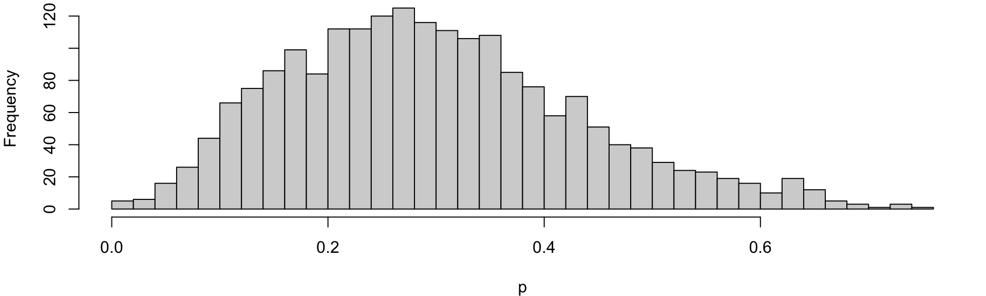
Example: Let \(p\) be the proportion of customers who choose oat milk instead of diary. We might model: \[ p \sim \text{Beta}(\alpha=3, \beta=7) \]

The parameters can be interpreted as:

  • you expect ~30% of customers to choose oat milk (prior mean = 0.3)
  • but you are not very certain (small \(\alpha + \beta = 10\))
set.seed(12); b <- rbeta(2000, shape1 = 3, shape2 = 7)
mean(b)
[1] 0.2970271
par(mar=c(4,4,0,1)); hist(b, breaks = 30, main = "", xlab = "p")

Example (extended): Continue from the previous example, suppose that during the morning rush, the barista records 20 customers. Among these, 9 chose oat milk and 11 chose daily. This is Binomial data:

\[ X \,|\, p \sim \text{Binomial}(n=20, p), \]

where \(X\) is the number of oat-milk orders out of 20 and \(p\) is the true (but unknown) probability a customer chooses oat milk.

You observe \(X,\) but you don’t know \(p.\) Bayesian thinking is about learning what \(p\) might be.

So, we give \(p\) a prior distribution (prior belief):

\[ p \sim \text{Beta}(\alpha=3, \beta=7) \]

With the data, we can update your belief using Bayes’ rule:

\[ f(p \,|\, X) = \frac{f(X\,|\,p)f(p)}{f(X)} \qquad \equiv \qquad \text{Posterior} = \frac{\text{Likelihood}\times\text{Prior}}{\text{Evidence}}. \]

  • Likelihood is from Binomial: \(\displaystyle f(X|p)= {20 \choose X} p^X(1-p)^{20-X}.\)
  • Prior is from Beta: \(f(p) \propto p^{\alpha-1}(1-p)^{\beta-1}.\)

\[ \text{Likelihood}\times\text{Prior}:\;\;f(X\,|\,p)f(p) \propto p^{X+\alpha-1}(1-p)^{(20-X)+\beta-1} \]

The expression \[ \text{Likelihood}\times\text{Prior}:\;\;f(X\,|\,p)f(p) \propto p^{X+\alpha-1}(1-p)^{(20-X)+\beta-1} \]

is exactly the kernel of a Beta distribution. So the posterior must be

\[ p \,|\, X \sim \text{Beta}(\alpha+X, \beta+(20-X)) \]

Since the number of oat-milk orders \(X\) is 9. Then,

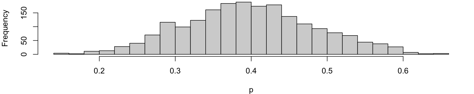
\[ p \,|\, X \sim \text{Beta}(12, 18). \]

set.seed(13); b <- rbeta(2000, shape1 = 12, shape2 = 18)
mean(b)
[1] 0.3982516
par(mar=c(4,4,0,1)); hist(b, breaks = 30, main = "", xlab = "p")

The posterior mean is 0.4, so our belief shifts from 30% to 40%.

Part 2: Joint distributions and dependence

Why dependence matters in simulation

In real systems, random variables rarely act alone.

Examples:

  • High arrival rate → longer waiting times
  • High demand → longer service times (fatigue, overload)
  • High rainfall → high river levels
  • High market return → high portfolio return

Incorrectly assuming independence can lead to:

  • Underestimated variance
  • Biased risk estimates
  • Unrealistic system behaviour

Simulation provides flexibility to incorporate complex dependence structures — but only if we understand the joint distribution.

Joint distributions

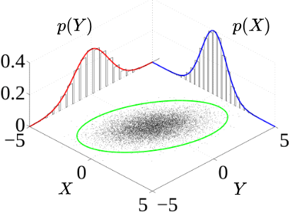
Figure 1: Joint probability distribution samples (black) and marginal densities (blue and red)

  • The surface is the joint density \(f_{X,Y}(x,y)\).
  • The curves along the axes are the marginals \(f_X(x)\) and \(f_Y(y)\).
  • The scatter cloud (in green circle) shows sample points from the joint distribution.

A joint distribution is a multivariate distribution. It is the probability structure that describes how several random variables behave together.

  • For two variables \(X\) and \(Y\), the joint distribution \(f_{X,Y}(x,y)\) is a bivariate distribution.

  • For \(k\) variables, \(X_1, \dots, X_k\), the joint distribution \(f_{X_1,\dots ,X_k}(x_1,\dots ,x_k)\) is a multivariate distribution.

Discrete case

Joint PMF \(p(x,y) = P(X=x, Y=y), \qquad p(x,y) \ge 0, \qquad \sum_x \sum_y p(x,y) = 1.\)
Joint CDF \(F_{XY}(x,y) = P(X\leq x, Y\leq y) = \sum_{x_i \leq x}\sum_{y_j \leq y} p(x_i, y_j).\)
Marginals \(p_X(x) = \sum_y p(x,y), \qquad p_Y(y) = \sum_x p(x,y).\)


Continuous case

Joint PDF \(f(x,y), \qquad f(x,y) \ge 0, \qquad \int_{-\infty}^{\infty} \int_{-\infty}^{\infty} f(x,y)\,dx\,dy = 1.\)
Joint CDF \(F(x,y) = P(X \le x, Y \le y) = \int_{-\infty}^{x} \int_{-\infty}^{y} f_{X,Y}(u,v)\, dv\, du.\)
Marginals \(f_X(x) = \int f(x,y)\,dy, \qquad f_Y(y) = \int f(x,y)\,dx.\)


Mixed case: \(X \in \{1,2,\dots,k\}, \quad Y \text{ continuous}\)

Joint distribution \(f_{X,Y}(x,y) = P(X=x)\, f_{Y\mid X}(y \mid x), \qquad x=1,\dots,k.\)
Joint CDF \(F_{X,Y}(x,y) = P(X \le x,\, Y \le y) = \sum_{x_i \le x} P(X=x_i)\, F_{Y\mid X}(y \mid x_i).\)
Marginals \(P(X=x) = \int_{-\infty}^{\infty} f_{X,Y}(x,y)\,dy \qquad f_Y(y) = \sum_{x=1}^k f_{X,Y}(x,y).\)

Independence

The case in which the variables do not influence each other at all.

\(X\) and \(Y\) are independent \(\forall x,y\) if

\[p(x,y) = p_X(x)p_Y(y) \qquad \text{(discrete)}\\ f(x,y) = f_X(x)f_Y(y) \qquad \text{(continuous)}\]

Discrete Case Example

Let \(X\) and \(Y\) be two discrete independent random variables

  • \(X\sim \mathrm{Bernoulli}(0.5)\) and
  • \(Y\sim \mathrm{Bernoulli}(0.3).\)

Because \(X\) and \(Y\) are independent, we simulate them separately.

set.seed(123)
n <- 5000
X <- rbinom(n, 1, 0.5)
Y <- rbinom(n, 1, 0.3)
cor(X, Y)
[1] -0.01700378

The correlation is close to 0.

Continuous Case Example

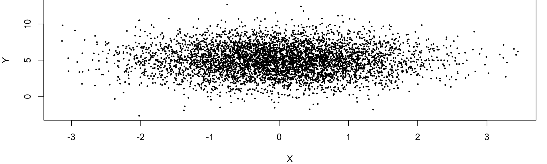
Let X and Y be continuous independent random variables \(X\sim \mathcal{N}(0,1)\) and \(Y\sim \mathcal{N}(5,4)\)

Because of independence:

\[f_{X,Y}(x,y)=f_X(x)\, f_Y(y)=\frac{1}{\sqrt{2\pi }}e^{-x^2/2}\times \frac{1}{\sqrt{8\pi }}e^{-(y-5)^2/8}\]

set.seed(123); X <- rnorm(5000, 0, 1); Y <- rnorm(5000, 5, 2)
cor(X, Y)   # close to 0
[1] -0.00598005
par(mar = c(4,4,0,1)); plot(X, Y, pch=16, cex=0.4)

The scatterplot looks like a round cloud, with no directional trend.

Conditional distributions

But most real systems are not independent. In practice, we often observe one variable first and then ask:

How does this information affect the behaviour of the other variable?

Dependence is formalised through conditional distributions.

\[ P(X=x \mid Y=y) = \frac{p(x,y)}{p_Y(y)}, \quad p_Y(y)>0 \qquad \text{(discrete)} \\ f_{X|Y}(x \mid y) = \frac{f(x,y)}{f_Y(y)}, \quad f_Y(y)>0\qquad \text{(continuous)} \]

Recall that independence was defined by

\[ f(x,y) = f_X(x) f_Y(y). \]

Rewriting this gives

\[ f_{Y|X}(y \mid x) = \frac{f(x,y)}{f_X(x)}. \]

If independence holds, then

\[ f_{Y|X}(y \mid x)=f_Y(y). \]

Discrete Case Example


Suppose a small coffee shop with two types of customers:

  • Type A customers are quick to serve 60% of a time.
  • Type B customers take longer to order 40% of a time.

Let \(X\) be customer type, where \(X=0\) and \(X=1\) denote customer Type A and Type B, respectively.

Let \(Y\) be number of ordered completed in the next hour.

  • If the customer is Type A, baristas complete more orders (higher success probability; 70%).
  • If the customer is Type B, baristas complete fewer orders (lower success probability; 40%).

We model:

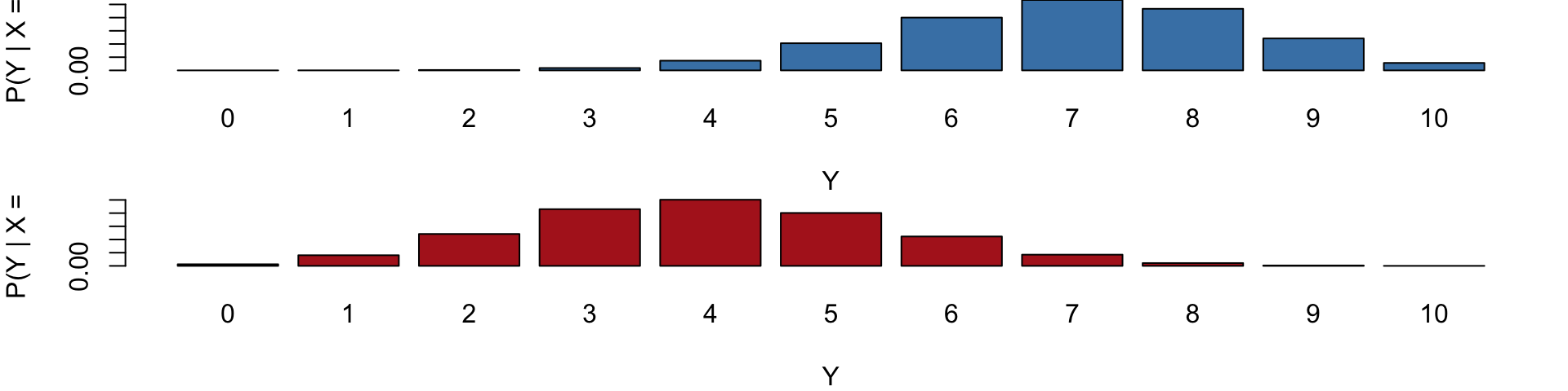
\[ Y\mid X=0\sim \mathrm{Binomial}(n=10,p=0.7), \\ Y\mid X=1\sim \mathrm{Binomial}(n=10,p=0.4) \]


This creates dependence between \(X\) and \(Y\).


Even if we know the marginal distribution of \(X\) and the marginal distribution of \(Y\), we cannot simulate the system correctly without the conditional structure.

set.seed(123)
X <- rbinom(5000, size = 1, prob = 0.4)   # 40% Type B customers
Y <- ifelse(
  X == 0,
  rbinom(n, size = 10, prob = 0.7),    # Type A
  rbinom(n, size = 10, prob = 0.4)     # Type B
)
cor(X, Y)
[1] -0.7032966
Code
y <- 0:10
pmf_A <- dbinom(y, size = 10, prob = 0.7)   # X = 0 (Type A)
pmf_B <- dbinom(y, size = 10, prob = 0.4)   # X = 1 (Type B)

# Set up side-by-side plotting area
par(mfrow = c(2, 1), mar = c(4, 4, 0, 1))

# PMF for X = 0
barplot(
  pmf_A,
  names.arg = y,
  col = "steelblue",
  main = "",
  xlab = "Y",
  ylab = "P(Y | X = 0)",
  ylim = c(0, max(pmf_A, pmf_B))
)

# PMF for X = 1
barplot(
  pmf_B,
  names.arg = y,
  col = "firebrick",
  main = "",
  xlab = "Y",
  ylab = "P(Y | X = 1)",
  ylim = c(0, max(pmf_A, pmf_B))
)
  • \(P(Y \mid X=0)\) (Type A) are concentrated at higher values of Y, meaning baristas complete more order on average.
  • \(P(Y \mid X=1)\) (Type B) shifts downward, with higher probability on smaller values of \(Y\).
  • Note: the value of \(X\) changes the entire shape of the distribution of \(Y\), not just its mean (dependency).

Continuous Case Example

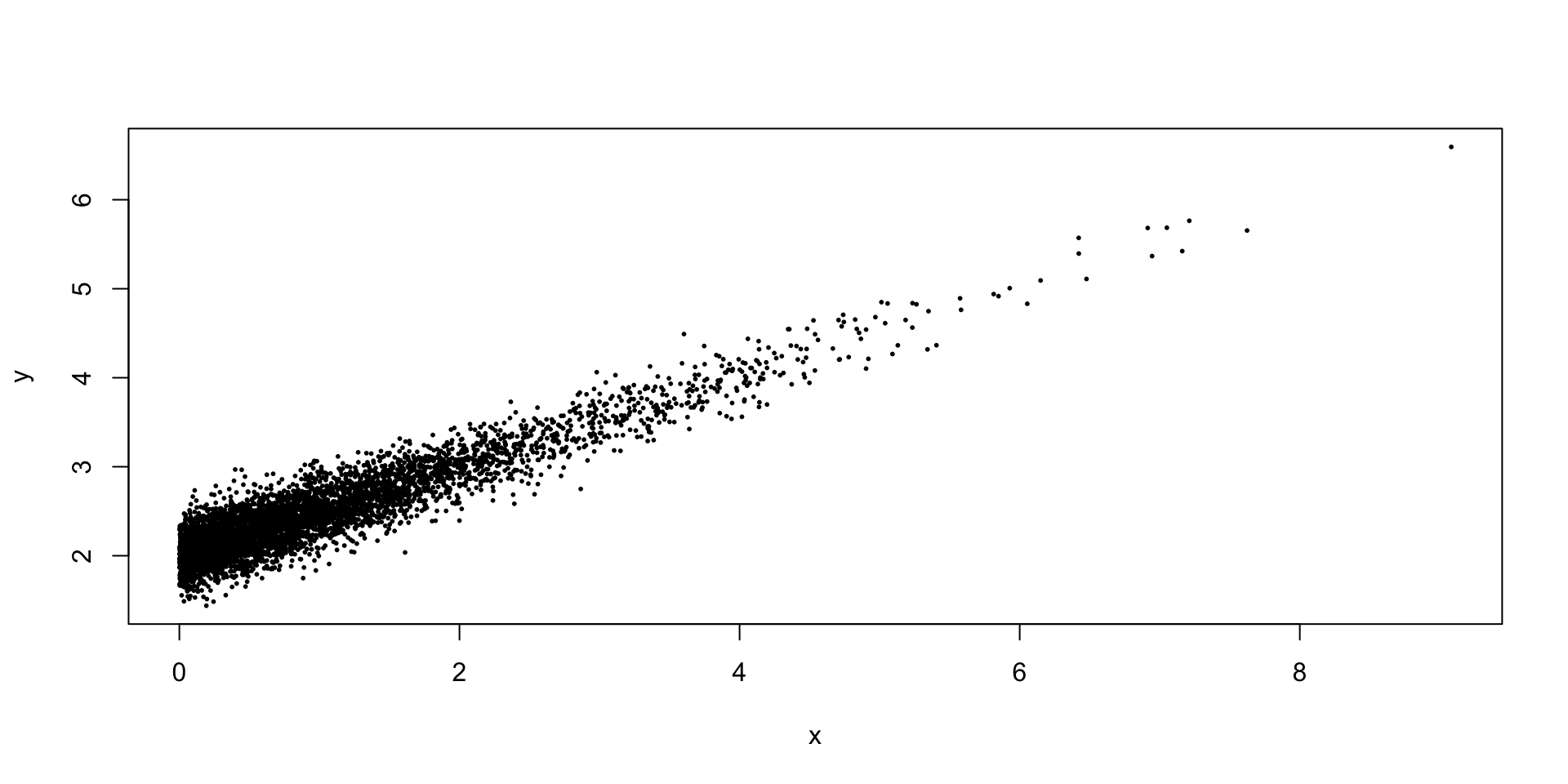
Suppose interarrival time \(X\) of a coffee shop influences service time \(Y\), such that

\[Y = 2 + 0.5X + \varepsilon,\]

where

\[X \sim \text{Exp}(1), \quad \varepsilon \sim N(0, 0.2^2),\]

and \(X\) and \(\varepsilon\) are independent.

Here:

  • When customers arrive slowly (large \(X\)), baristas work more carefully.
  • When arrivals are rapid (small \(X\)), service is faster.
set.seed(123)
x <- rexp(5000, rate = 1)
eps <- rnorm(n, mean = 0, sd = 0.2)
y <- 2 + 0.5*x + eps
cor(x, y)
[1] 0.9287826

Very high correlation.

plot(x, y, pch=16, cex=0.4)

The scatterplot reveals a clear linear trend, and the correlation is positive.

Even if we know the distribution of \(X\) and the distribution of \(Y\), without their joint structure we cannot simulate the system correctly.

Covariance and correlation

To quantify linear dependence, we define the covariance:

\[\mathrm{Cov}(X,Y) = \mathbb{E}\left[(X-\mathbb{E}[X])(Y-\mathbb{E}[Y])\right].\]

An equivalent expression is

\[\mathrm{Cov}(X,Y) = \mathbb{E}[XY] - \mathbb{E}[X]\mathbb{E}[Y].\]

If \(X\) and \(Y\) are independent, then

\[\mathrm{Cov}(X,Y) = 0.\]

The correlation coefficient is

\[\rho = \frac{\mathrm{Cov}(X,Y)}{\sigma_X \sigma_Y},\]

which lies in \([-1,1]\).

  • Correlation measures linear association but does not fully describe dependence.

  • Two variables may be uncorrelated yet dependent — an important subtlety in simulation modelling.

When to use covariance


Covariance is useful when you care about the direction of the relationship.

Covariance answers:

“Do X and Y increase together or move in opposite directions?”

But the magnitude is not interpretable, because it depends on the units of X and Y.


When to use correlation


Correlation is the standardised version of covariance. It removes units and rescales the relationship to the familiar range [-1,1].

Correlation answers:

“How strong is the linear relationship between X and Y, on a universal scale?”

Because it’s standardised, you can compare height vs weight, income vs education, temperature vs electricity use, etc, even though all are in different units.

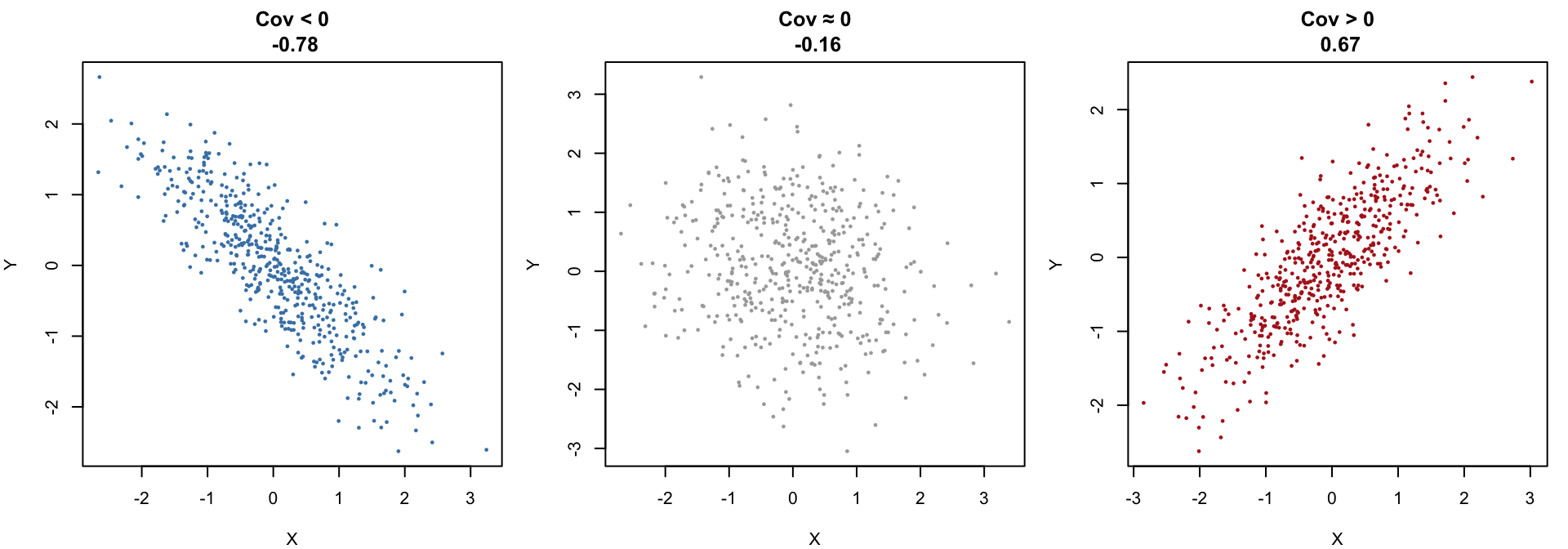
The sign of the covariance of two random variables X and Y

Code
set.seed(123)

par(mfrow = c(1, 3), mar = c(4, 4, 3, 1))

### 1. Negative covariance
x1 <- rnorm(500)
y1 <- -0.8 * x1 + rnorm(500, sd = 0.5)
plot(x1, y1,
     pch = 16, cex = 0.5, col = "steelblue",
     main = paste("Cov < 0\n", round(cov(x1, y1), 2)),
     xlab = "X", ylab = "Y")

### 2. Approximately zero covariance
x2 <- rnorm(500)
y2 <- rnorm(500)
plot(x2, y2,
     pch = 16, cex = 0.5, col = "darkgray",
     main = paste("Cov ≈ 0\n", round(cov(x2, y2), 2)),
     xlab = "X", ylab = "Y")

### 3. Positive covariance
x3 <- rnorm(500)
y3 <- 0.8 * x3 + rnorm(500, sd = 0.5)
plot(x3, y3,
     pch = 16, cex = 0.5, col = "firebrick",
     main = paste("Cov > 0\n", round(cov(x3, y3), 2)),
     xlab = "X", ylab = "Y")
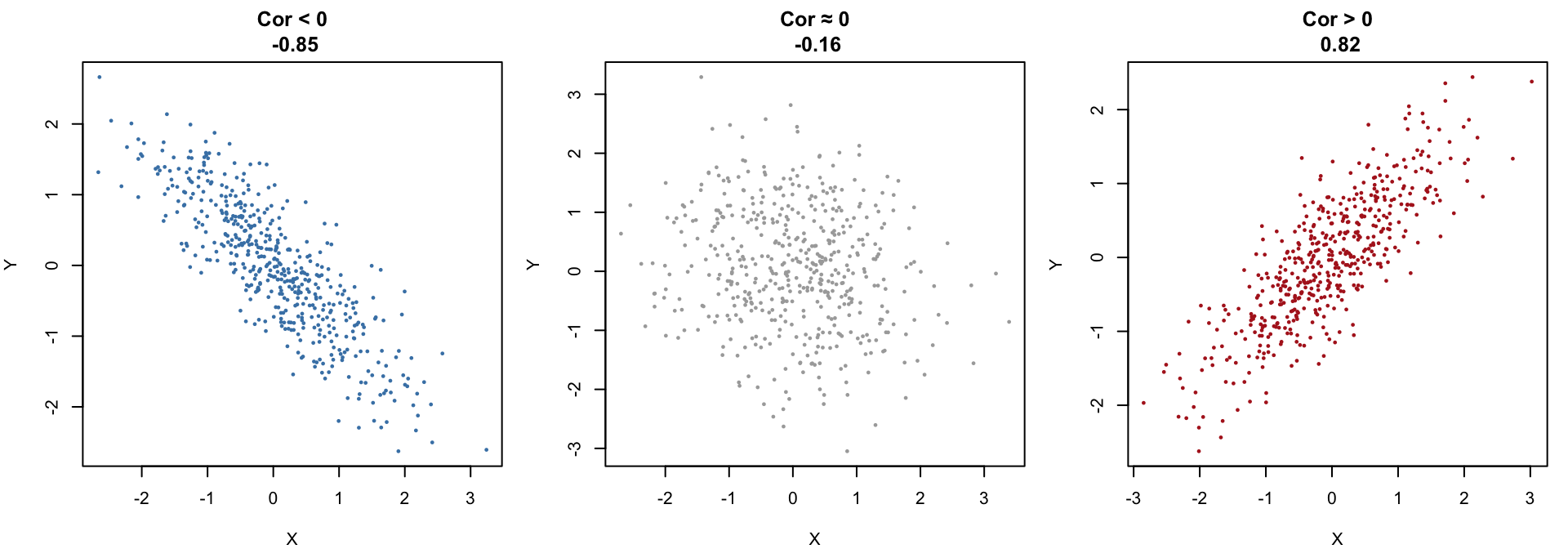
  • \(Cov(X, Y) < 0\) shows a clear downward trend. As X increases, Y tends to decrease.
  • \(Cov(X, Y) ≈ 0\) shows a round, structureless cloud — classic independence‑looking scatter.
  • \(Cov(X, Y) > 0\) shows a clear upward trend. As X increases, Y tends to increase.

The sign of the correlation of two random variables X and Y

Code
set.seed(123)

par(mfrow = c(1, 3), mar = c(4, 4, 3, 1))

### 1. Negative correlation
x1 <- rnorm(500)
y1 <- -0.8 * x1 + rnorm(500, sd = 0.5)
plot(x1, y1,
     pch = 16, cex = 0.5, col = "steelblue",
     main = paste("Cor < 0\n", round(cor(x1, y1), 2)),
     xlab = "X", ylab = "Y")

### 2. Approximately zero correlation
x2 <- rnorm(500)
y2 <- rnorm(500)
plot(x2, y2,
     pch = 16, cex = 0.5, col = "darkgray",
     main = paste("Cor ≈ 0\n", round(cor(x2, y2), 2)),
     xlab = "X", ylab = "Y")

### 3. Positive correlation
x3 <- rnorm(500)
y3 <- 0.8 * x3 + rnorm(500, sd = 0.5)
plot(x3, y3,
     pch = 16, cex = 0.5, col = "firebrick",
     main = paste("Cor > 0\n", round(cor(x3, y3), 2)),
     xlab = "X", ylab = "Y")
  • \(\rho_{XY} < 0\) indicates a clear downward linear trend: as \(X\) increases, \(Y\) tends to decrease.

  • \(\rho_{XY} \approx 0\) produces a round, structureless cloud of points with no visible upward or downward tilt — the classic “no linear association” look.

  • \(\rho_{XY} > 0\) indicates a clear upward linear trend: as \(X\) increases, \(Y\) tends to increase.

Special Case: Bivariate normal distribution


A central example in simulation is the bivariate normal distribution. A bivariate normal distribution is a two‑dimensional version of the normal distribution. It describes the joint behaviour of two continuous random variables, usually written as:

\[(X,Y)\sim \mathrm{BVN}(\mu _X,\mu _Y,\sigma _X^2,\sigma _Y^2,\rho )\]

or

\[\begin{pmatrix} X \\ Y \end{pmatrix} \sim N \left( \begin{pmatrix} \mu_X \\ \mu_Y \end{pmatrix}, \begin{pmatrix} \sigma_X^2 & \rho \sigma_X \sigma_Y \\ \rho \sigma_X \sigma_Y & \sigma_Y^2 \end{pmatrix} \right)\]

It is fully determined by five parameters:

  • mean of \(X\): \(\mu _X\)
  • mean of \(Y\): \(\mu _Y\)
  • variance of \(X\): \(\sigma _X^2\)
  • variance of \(Y\): \(\sigma _Y^2\)
  • correlation between \(X\) and \(Y\): \(\rho\)

Here, the parameter \(\rho\) controls linear dependence.

Key properties

  1. Each marginal is normal \(\quad X\sim N(\mu _X,\sigma _X^2),\qquad Y\sim N(\mu _Y,\sigma _Y^2)\)

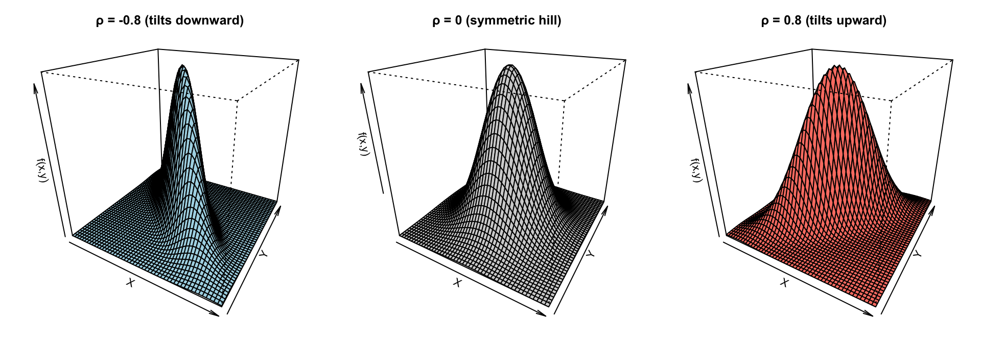
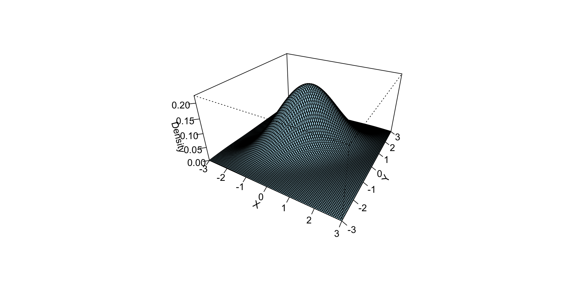
  2. The joint density forms a 3D bell surface The height of the surface at point \((x,y)\) is the joint density \(f_{X,Y}(x,y).\) The shape of this surface depends heavily on the correlation \(\rho:\)

  3. Contours are ellipses. If you slice the 3D surface horizontally, you get ellipses. The orientation of the ellipse tells you the sign of the correlation.

  4. Independence happens only when \(\rho =0\). This is not true for most distributions. It’s a unique property of the multivariate normal family.

3D bivariate normal surfaces for different correlations
library(mvtnorm)

# Grid for evaluation
x <- seq(-3, 3, length = 50)
y <- seq(-3, 3, length = 50)
grid <- expand.grid(x = x, y = y)

# Function to compute BVN density matrix
bvn_matrix <- function(rho) {
  Sigma <- matrix(c(1, rho, rho, 1), 2, 2)
  z <- dmvnorm(grid, mean = c(0, 0), sigma = Sigma)
  matrix(z, nrow = length(x), ncol = length(y))
}

z_neg <- bvn_matrix(-0.8)
z_zero <- bvn_matrix(0)
z_pos <- bvn_matrix(0.8)

par(mfrow = c(1, 3), mar = c(2, 2, 3, 1))

# 1. Negative correlation
persp(x, y, z_neg,
      theta = 30, phi = 25,
      col = "lightblue",
      main = "ρ = -0.8 (tilts downward)",
      xlab = "X", ylab = "Y", zlab = "f(x,y)")

# 2. Zero correlation
persp(x, y, z_zero,
      theta = 30, phi = 25,
      col = "lightgray",
      main = "ρ = 0 (symmetric hill)",
      xlab = "X", ylab = "Y", zlab = "f(x,y)")

# 3. Positive correlation
persp(x, y, z_pos,
      theta = 30, phi = 25,
      col = "salmon",
      main = "ρ = 0.8 (tilts upward)",
      xlab = "X", ylab = "Y", zlab = "f(x,y)")

We can simulate correlated normals using a linear transformation.

set.seed(123)
rho <- 0.8
z1 <- rnorm(5000)
z2 <- rnorm(5000)
x <- z1
y <- rho*z1 + sqrt(1 - rho^2)*z2
cor(x, y)
[1] 0.7963105
Code
# Define parameters
rho <- 0.7

# Create grid
x <- seq(-3, 3, length = 100)
y <- seq(-3, 3, length = 100)
grid <- expand.grid(x = x, y = y)

# Bivariate normal density (mean=0, var=1)
f <- function(x, y, rho) {
  1/(2*pi*sqrt(1 - rho^2)) *
    exp(-(x^2 - 2*rho*x*y + y^2) / (2*(1 - rho^2)))
}

# Compute density values
z <- matrix(f(grid$x, grid$y, rho), nrow = 100)

# 3D perspective plot
persp(x, y, z,
      theta = 30, phi = 30,
      expand = 0.5,
      col = "lightblue",
      xlab = "X",
      ylab = "Y",
      zlab = "Density",
      ticktype = "detailed")