STAT2005 Computer Simulation

Lecture 5 — Simulation of Continuous Random Variables

Sam Wiwatanapataphee (275287a@curtin.edu.au)

26 Mar 2026

Goals today


  • Part 1: Transformation Methods (Extended)
    • Transformation of a Single Random Variable
      • Discrete Case
      • Continuous Case
        • Monotone Transformations
        • Non-Monotone Transformations
    • Inverse Transform Sampling
      • Exponential Distribution Example
        (Closed-form Inverse CDF)
      • Quadratic CDF Example
      • Normal Distribution Example
        (No Closed-form Inverse CDF)
      • Cubic Polynomial CDF Example
      • Limitations of Inverse Transform
  • Part 2: The Acceptance-Rejection Methods
    • General Acceptance-Rejection Algorithm
    • Cubic Polynomial CDF Example
      (Continue from Part 1)
    • Normal-Cauchy Example


  • Part 3: Precision of Simulation Result (Revision)
    • Monte Carlo Estimation

Part 1: Transformation of Random Variables

Recap: Where We Are So Far

  • We use simulation to study random systems by repeating experiments many times
  • To simulate, we need to generate random variables
  • Random variables follow probability distributions

The Key Building Block

  • Computers generate pseudo-random numbers
  • In practice, we generate reproducible rvs: \(\boxed{U \sim \text{Uniform}(0,1)}\)
  • Then, we used simple rules to generate random variables:

Bernoulli(p)

Generate \(U \rightarrow\) If \(U < p\), return 1, else return 0

Discrete Distributions:

Use the precision method or the inverse CDF method

  • Idea: Start with Uniform(0,1), then transform it.
  • How do we generate any other distribution? Exponention? Normal? Custom distributions?

Transformation of a Single Random Variable

When we apply a function to a random variable, the result is itself a new random variable. If \(X\) has a known distribution and we define
\[ Y = g(X), \]

then the key question is: What is the distribution of \(Y\)?

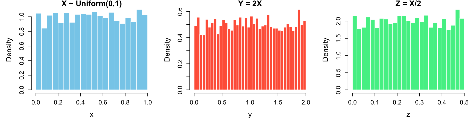
Suppose \(X \sim \text{Uniform}(0,1)\) and \(Y = 2X, Z = X/2.\)
set.seed(1234)

x <- runif(5000, 0, 1)
y <- 2 * x
z <- x / 2

par(mfrow = c(1, 3), mar = c(4,5,1,1))

hist(x, prob = TRUE, breaks = 30,
     main = "X ~ Uniform(0,1)", xlab = "x",
     col = "skyblue", border = "white",
     cex.lab = 1.4, cex.main = 1.5, cex.axis = 1.2)

hist(y, prob = TRUE, breaks = 30,
     main = "Y = 2X", xlab = "y",
     col = "tomato", border = "white",
     cex.lab = 1.4, cex.main = 1.5, cex.axis = 1.2)

hist(z, prob = TRUE, breaks = 30,
     main = "Z = X/2", xlab = "z",
     col = "seagreen2", border = "white",
     cex.lab = 1.4, cex.main = 1.5, cex.axis = 1.2)

  • If \(Y = 2X \rightarrow\) values spread out (stretched) \(\rightarrow\) density becomes lower.
  • If \(Y = X/2 \rightarrow\) values squeezed (compressed) \(\rightarrow\) density becomes higher

🎯 Key idea: Probability is conserved, but density is redistributed

Discrete Case (Intuition)

When we transform a random variable, \(Y = g(X),\) multiple values of \(X\) may map to the same value of \(Y\).

The probability of \(Y\) is obtained by collecting contributions from all such values:

\[ p_Y(y) = \sum_{x : g(x) = y} p_X(x). \]

This is a “probability bookkeeping” rule: every value of \(Y\) inherits probability from the \(X\)-values that produce it.


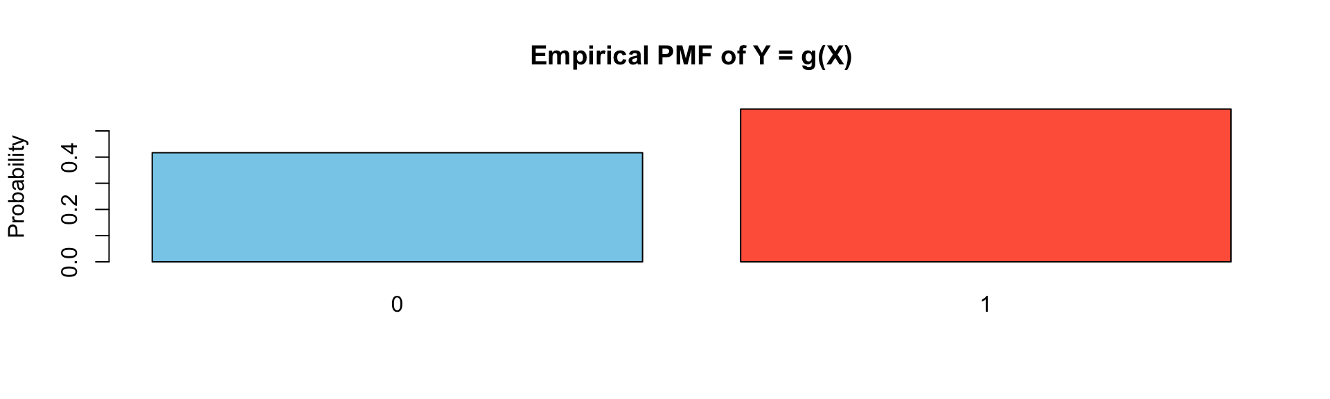
Example: Let \(X \in \{1,2,3,4\}\) with given probabilities

\[ P(X=1)=0.1,\quad P(X=2)=0.2, \]

\[ P(X=3)=0.3,\quad P(X=4)=0.4. \]

Define:

\[ Y = \begin{cases} 0 & \text{if } X \text{ is odd} \\ 1 & \text{if } X \text{ is even} \end{cases} \]

Then:

\[ Y = 0: \text{from } X = 1,3 \qquad Y = 1: \text{from } X = 2,4 \]

PMF of \(Y:\)

\[ P(Y=0)=P(X=1)+P(X=3)=0.1+0.3=0.4, \]

\[ P(Y=1)=P(X=2)+P(X=4)=0.2+0.4=0.6 \]

set.seed(1234)

# Original discrete variable
X <- sample(1:4, size = 5000, replace = TRUE,
            prob = c(0.1, 0.2, 0.3, 0.4))

# Transformation
Y <- ifelse(X %% 2 == 1, 0, 1)

# Plot empirical pmf of Y
barplot(prop.table(table(Y)),
        col = c("skyblue", "tomato"),
        main = "Empirical PMF of Y = g(X)",
        ylab = "Probability")

Continuous Case

  • For discrete variables: we add probabilities.

  • For continuous variables: \(\boxed{P(X = x) = 0.}\)

👉 We cannot “collect probabilities” anymore.

  • For continuous random variables, there are in principle two approaches:

CDF‑based Method

derives the distribution of \(Y\) by working with cumulative probabilities

PDF‑based Method

determines how density changes under the transformation


Key Idea: Density Transformation

  • Instead of probabilities, we work with density.

  • When we transform using \(Y = g(X)\), we must track how density is stretched or compressed.

    • stretches some regions → density decreases
    • compresses some regions → density increases
  • The adjustment is captured by a derivative.

flowchart LR
  %% Monotone transformation
  subgraph M["Monotone Y = g(X)"]
    direction TB
    x1["x₁"] -->|"g"| y1["y₁"]
    x2["x₂"] -->|"g"| y2["y₂"]
    x3["x₃"] -->|"g"| y3["y₃"]
  end

  %% Non-monotone transformation
  subgraph N["Non‑monotone Y = g(X)"]
    direction TB
    a1["x₁"] -->|"g"| b1["y₁"]
    a2["x₂"] -->|"g"| b2["y₂"]
    a3["x₃"] -->|"g"| b2
    a4["x₄"] -->|"g"| b3["y₃"]
  end

  %% Notes
  note1["Each y has exactly one preimage"]:::note
  note2["A y may have multiple preimages"]:::note

  M --- note1
  N --- note2

  %% Styling
  classDef note fill:#f5f5f5,stroke:#999,stroke-dasharray: 4 4,color:#111;

  style M fill:#f5f5f5,stroke:#999,stroke-dasharray: 4 4,color:#111;
  style N fill:#f5f5f5,stroke:#999,stroke-dasharray: 4 4,color:#111;

  %% Make all arrows black
  linkStyle default stroke:#000,stroke-width:1.5px;

Case 1: Monotone Transformations

  • If \(g\) is one-to-one and strictly increasing or decreasing, each value of \(Y\) comes from exactly one \(X.\)
  • Then, the PDF of \(Y\) is given by the change-of-variables formula,

\[ f_Y(y) = f_X(g^{-1}(y)) \left| \frac{d}{dy} g^{-1}(y) \right| \]

  • The derivative term adjusts for stretching/compression.

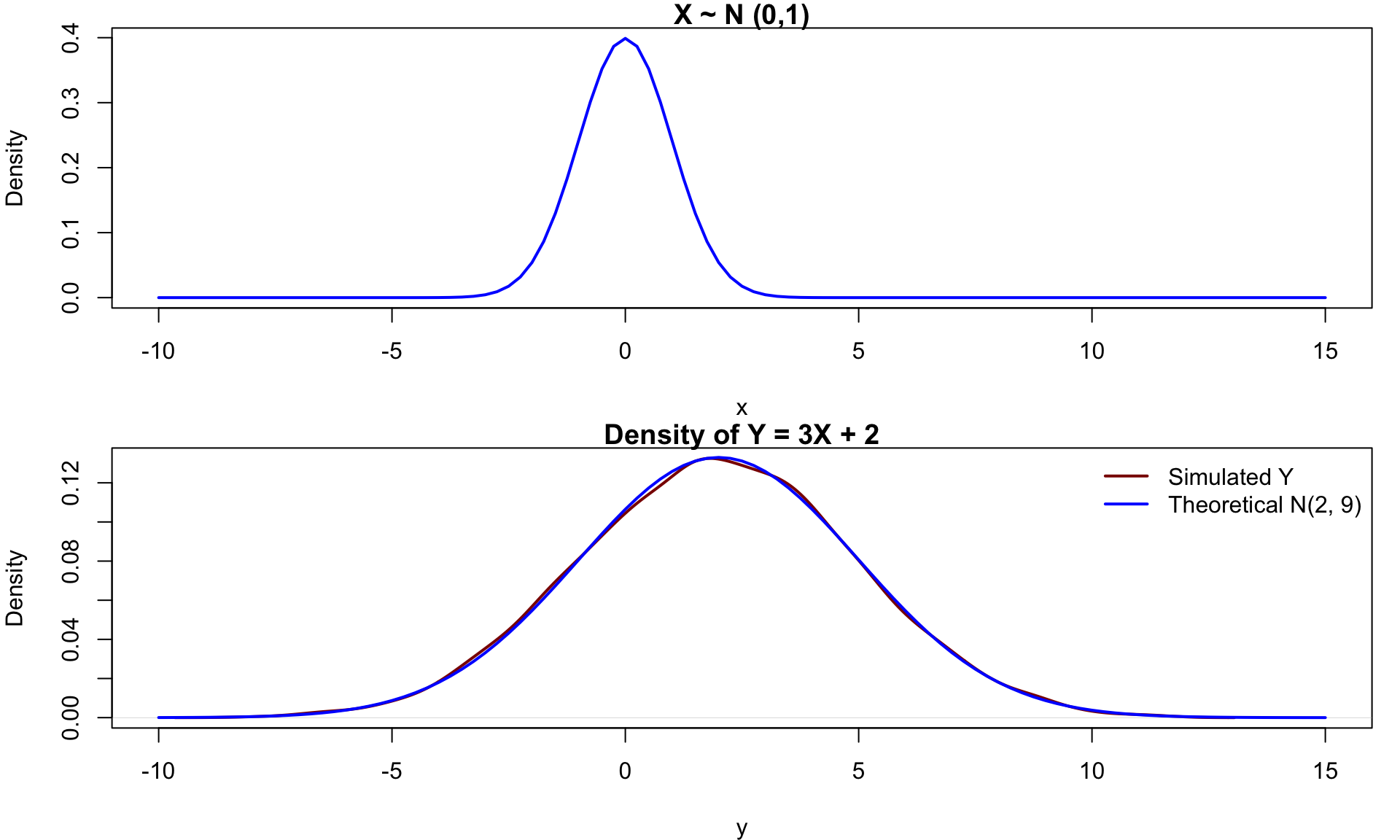
Example: Let \(X\sim \mathcal{N}(0,1)\) and define \(Y=3X+2\). Determine the PDF of \(Y\).

We know \(Y=g(X)=3X+2\), which is strictly increasing. The inverse is

\[ x=g^{-1}(y)=\frac{y-2}{3} \quad \text{and} \quad \frac{d}{dy}g^{-1}(y)=\frac{1}{3}. \]

The PDF of \(X\) is

\[f_X(x)=\frac{1}{\sqrt{2\pi }}e^{-x^2/2}.\]

By the change‑of‑variables formula,

\[ f_Y(y) = f_X\! \left( \frac{y-2}{3}\right) \cdot \frac{1}{3} =\frac{1}{3}\cdot \frac{1}{\sqrt{2\pi }}\exp \! \left( -\frac{1}{2}\left( \frac{y-2}{3}\right) ^2\right). \]

This is recognised as the PDF of \(\boxed{Y\sim \mathcal{N}(2,9)}.\)

Suppose \(X \sim N(0,1)\) and \(Y = 3X + 2\)
set.seed(1234)

# Original variable
X <- rnorm(5000)

# Transformation
Y <- 3*X + 2

par(mfrow = c(2,1), mar = c(4,4,1,1))

# Theoretical X ~ N(0,1)
curve(dnorm(x, mean = 0, sd = 1), from = -10, to = 15, col = "blue", lwd = 2,
     xlab = "x", ylab = "Density", main = "X ~ N (0,1)")

# Plot simulated density
plot(density(Y), xlim =c(-10, 15),
     col = "darkred", lwd = 2,
     main = "Density of Y = 3X + 2",
     xlab = "y")

# Add theoretical curve
curve(dnorm(x, mean = 2, sd = 3),
      col = "blue", lwd = 2, add = TRUE)

legend("topright",
       legend = c("Simulated Y", "Theoretical N(2, 9)"),
       col = c("darkred", "blue"), lwd = 2, bty = "n")
  • Because \(Y=3X+2\) stretches the values of \(X\), the density becomes more spread out (lower peak).

  • To preserve total probability, the density is scaled by the derivative term in the change-of-variables formula:

    \[ \left| \frac{dx}{dy} \right| = \frac{1}{3}. \]

Aside: Change-of-variables Formula (Intuition)

Key Idea: Probability is preserved under transformation, i.e.

\[ P(a \leq Y \leq b) = P(g^{-1}(a) \leq X \leq g^{-1}(b)) \]

To understand how density changes, we look at a small interval:

\[ P(y \leq Y \leq y + dy) = P(x \leq X \leq x + dx), \tag{1} \]

where \(\boxed{x = g^{-1}(y)}.\) From the local linear approximation (calculus), we have

\[ dx \approx \frac{dx}{dy}dy. \]

For very small intervals, probability is approximately: (probability ≈ density × width). Then,

\[ \begin{aligned} P(y \leq Y \leq y + dy) &\approx f_Y(y)\;dy, \\ P(x \leq X \leq x + dx) &\approx f_X(x)\;dx. \end{aligned} \tag{2} \]

From (1) and (2), we have

\[ \begin{aligned} f_Y(y) \; dy &= f_X(x) \; dx \\ f_Y(y) &= f_X(x)\frac{dx}{dy}, \end{aligned} \]

and since densities must be positive: \(\boxed{f_Y(y) = f_X(g^{-1}(y)) \left| \dfrac{d}{dy} g^{-1}(y) \right|}\)

Takeaway: The derivative term tells us how much the transformation stretches or compresses the space.

Case 2: Non-Monotone Transformations

  • If \(g\) is not one-to-one, multiple values of \(X\) map to the same \(Y.\)

  • Then we must add all contributions:

\[ f_Y(y) = \sum_{x : g(x) = y} f_X(x)\left|\frac{dx}{dy}\right| \]


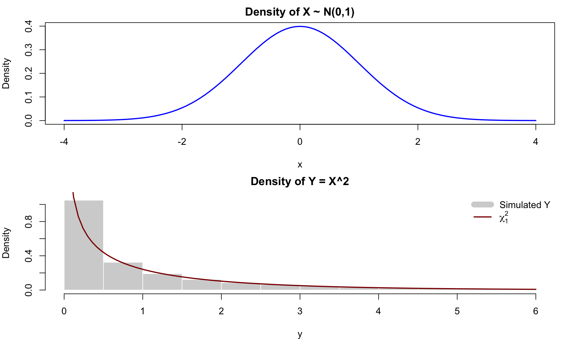
Example: Let \(X \sim \mathcal{N}(0,1)\) and define \(Y = X^2.\) Find the PDF of \(Y\).

  • For a given \(y\), two values map to it:

\[ x = \sqrt{y}, \quad x = -\sqrt{y} \]

  • Both contribute to the density
  • Using the non-monotone trasformation rule, we have:

\[ f_Y(y) = \frac{1}{\sqrt{2\pi}}e^{-y/2}\cdot\frac{1}{\sqrt{y}}. \]

  • This is recognised as the PDF of a Chi-squared distribution with 1 degree of freedom, i.e. \(\boxed{Y \sim \chi^2_1}\)
Suppose X ~ N(0,1) and Y = X^2
set.seed(1234)

# Original variable
X <- rnorm(5000)

# Transformation
Y <- X^2

op <- par(mfrow = c(2,1), mar = c(4,4,2,1))

# Panel 1: X ~ N(0,1)
curve(dnorm(x, mean = 0, sd = 1),
      from = -4, to = 4,
      col = "blue", lwd = 2,
      xlab = "x", ylab = "Density",
      main = "Density of X ~ N(0,1)")

# Panel 2: Y = X^2
hist(Y, breaks = 40, freq = FALSE,
     col = "lightgray", border = "white",
     xlim = c(0, 6), ylim = c(0, 1.1),
     main = "Density of Y = X^2",
     xlab = "y", ylab = "Density")

curve(dchisq(x, df = 1),
      from = 1e-4, to = 6,
      col = "darkred", lwd = 2, add = TRUE)

legend("topright",
       legend = c("Simulated Y", expression(chi[1]^2)),
       col = c("lightgray", "darkred"),
       lwd = c(10, 2), bty = "n")
  • \(X \sim N(0,1)\) distribution spreads across both negative and positive values.
  • \(Y = X^2\) distribution is right-skewed (non-negative).

Why Transformation Matters to Simulation

So far:

We start with \(X\)
Apply transformation \(Y = g(X)\)
Find distribution of \(Y\)


Now we reverse the idea:

Start with \(U \sim \text{Uniform}(0,1)\)
Choose \(g\) to create a desired distribution


👉 Goal:

\[ X = g(U) \]

so that \(X\) has the distribution we want

How do we find such a transformation \(g\)?

Use the CDF

This leads to

Inverse Transform Sampling

Inverse Transform Sampling

Every random variable has a CDF:

\[ F_X(x) = P(X \le x) \]

The CDF maps values of \(X\) → probabilities in (0,1)

👉 This suggests a connection to Uniform(0,1)

Probability Integral Transform

If \(X\) has CDF \(F_X\), then:

\[ U = F_X(X) \sim \text{Uniform}(0,1) \]

👉 The CDF transforms any distribution → Uniform(0,1)

then reversing gives:

\[ \boxed{X = F_X^{-1}(U), \quad U \sim \text{Uniform}(0,1)} \]

which is known as the sampling rule.

To simulate \(X \sim F_X\):

Generate \(U \sim \text{Uniform}(0,1)\)
Transform: \(X = F_X^{-1}(U)\)

Exponential Distribution Example (Closed-form Inverse CDF)

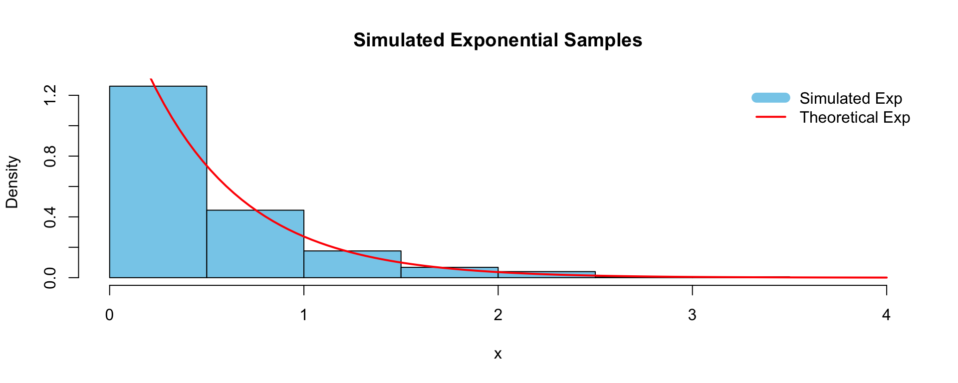
Let \(X \sim \text{Exp}(\lambda)\) with the following CDF:

\[ F(x) = 1 - e^{-\lambda x} \]

Setting \(U = F(X)\) and solving for \(X\) gives the inverse term:

\[ X = -\frac{1}{\lambda} \log(1 - U), \quad U \sim \text{Uniform}(0,1). \]

X ~ Exp(\(\lambda=2\))
set.seed(1234)

u <- runif(1000)
lambda <- 2

x <- -log(1 - u) / lambda

hist(x, prob = TRUE, col = "skyblue",
     main = "Simulated Exponential Samples")

curve(dexp(x, rate = lambda),
      col = "red", lwd = 2, add = TRUE)

legend("topright",
       legend = c("Simulated Exp", "Theoretical Exp"),
       col = c("skyblue", "red"), lwd = c(10,2), bty = "n")

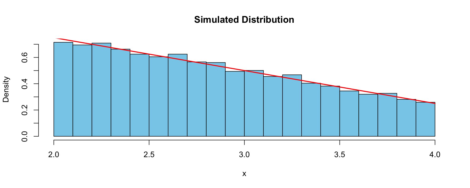
Quadratic CDF Example

Consider the electrical current distribution model where the pdf of \(X\) is given by

\[ f(x) = 1.25 - 0.25x, \quad 2 \leq x \leq 4. \]

Suppose a simulation of \(X\) is required as part of some larger system analysis.

Step 0: Check for valid PDF

\[ \int_2^4 (1.25 - 0.25x)\,dx = 1 \quad \rightarrow \quad \text{valid density.} \]

Step 1: Determine the CDF \(F(x)\)

\[ \begin{aligned} F(x) &= \int_2^x (1.25 - 0.25y)\,dy \\ &= \left[1.25y - 0.125y^2 \right]_2^x \\ F(x) &= 1.25x - 0.125x^2 - 2 \end{aligned} \]

Step 2: Determine the inverse CDF \(X=F^{-1}_X(U)\)

\[ \begin{aligned} u &= F(x) = 1.25 x - 0.125x^2 -2 \\ 0 &= x^2 - 10x + 16 + 8u \\ x &= 5 \pm \sqrt{9-8u} \end{aligned} \]

  • Since the support is \(2 \leq x \leq 4,\) the only root satisfies this is \(\boxed{x = 5 - \sqrt{9 - 8u}}.\)
  • \(\boxed{X = 5 - \sqrt{9 - 8U}}.\)
  • This transformation maps Uniform(0,1) values into the interval [2,4] with the correct shape.
set.seed(1234)
u <- runif(10000)
x <- 5 - sqrt(9 - 8 * u)

hist(x, prob = TRUE, col = "skyblue",
     main = "Simulated Distribution")

curve(1.25 - 0.25*x, add = TRUE, col = "red", lwd = 2)

Normal Distribution Example (No Closed-form Inverse CDF)

Recall the PDF of the standard normal distribution \(X \sim N(0,1):\)

\[ f(x)=\frac{1}{\sqrt{2\pi}}\exp{\left(-\frac{x^2}{2}\right)}, \quad x \in \mathbb{R}. \]

The CDF of \(X\) is \(\Phi(x):\)

\[ \Phi(x) = \frac{1}{\sqrt{2\pi}}\int_{-\infty}^x\exp{\left(-\frac{y^2}{2}\right)}\,dy, \]

has no closed-form expression.

  • The CDF has no closed-form expression, so neither does its inverse.
    • We must compute it numerically.
  • This is the reason why we use software or table to calculate Normal probabilities.

Cubic Polynomial CDF Example

\(F(x)\) is a polynomial function.

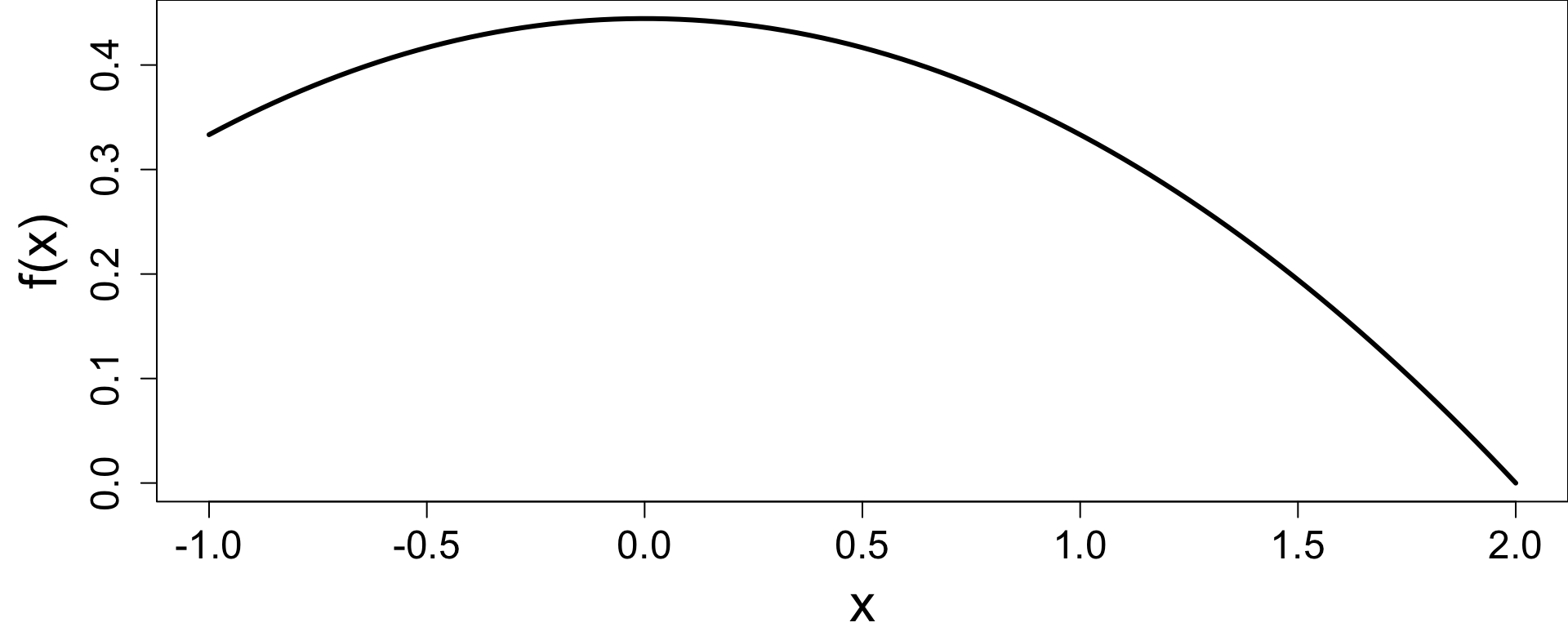
The measurement error \(X\) (in mV) of a particular volt-meter has the following distribution:

\[ f(x) = \begin{cases} \dfrac{4-x^2}{9}, & \quad -1 \leq x \leq 2 \\ 0, & \text{otherwise.} \end{cases} \]

The CDF is

\[ F(x) = \frac{-x^3+12x+11}{27}, \quad -1 \leq x \leq 2, \]

which is a cubic polynomial function.

  • It is not easy to solve for \(x = F^{-1}(u).\)

  • Numerical methods (e.d. Newton–Raphson) should be used to solve this kind of problem

When Does Inverse Transform Work?


Even if we can solve for inverse CDF, it may be:

  • slow
  • unstable
  • impractical in simulation

Case Difficulty
Exponential ✔ Easy (closed-form inverse)
Electrical example ✔ Moderate (quadratic)
Normal ❌ No closed-form inverse
Polynomial CDF ⚠️ Requires numerical methods


Note

👉 Not all distributions are equally tractable.

Limitations of Inverse Transform

No closed-form inverse

Many distributions (e.g. Normal) do not have an explicit inverse CDF.

Inversion can be difficult

Even when \(F(x)\) is known, solving \(u = F(x)\) may require numerical methods.

Computational cost

Numerical inversion can be slow or impractical in large simulations.

👉 We need more general methods that does not reqire \(F^{-1}\) and work for complex distributions.

  • Acceptance–Rejection Sampling
  • Specialised transformations such as Box–Muller for Normal simulation

Part 2: The Acceptance-Rejection Methods

Acceptance-Rejection Sampling

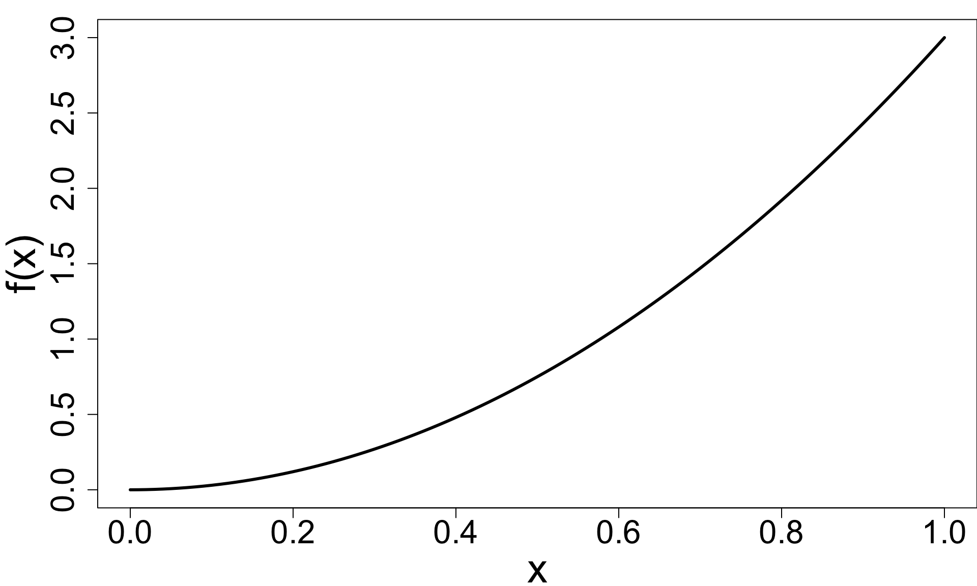
Example: We want to simulate

\[ f(x) = 3x^2, \quad 0 \le x \le 1, \]

which has increasing density with more weight near 1.

How do we simulate this?

First, check for valid PDF.

\[ \int_0^1 3x^2 \, dx = 1 \rightarrow \text{ valid PDF.} \]

Why Not Inverse Transform?

  • We would need \(X = F^{-1}(U).\)
  • Finding \(F(x)\) is easy, but inverting it is not simple.
  • 👉 Let’s try a different idea.
x <- seq(0, 1, length.out=100)
par(mar=c(4,5,1,0))
curve(3 * x^2, type = "l",
      lwd = 3, ylab = "f(x)",
      cex.axis=2, cex.lab=2.5)

Key Idea

  • Instead of transforming, we sample points in a region.
Draw a random point \((X, Y)\)
Accept it if it lies under the curve
  • 👉 This turns sampling into a geometry problem.

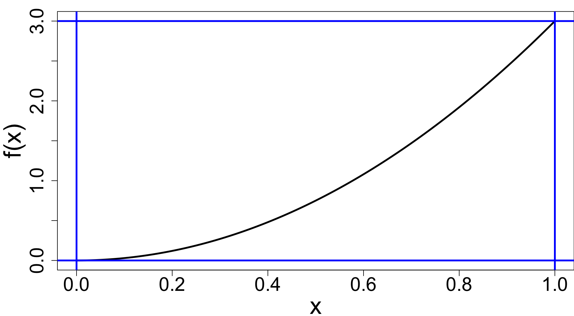
Visualisation

Consider the rectangle:

\[ 0 \le x \le 1, \quad 0 \le y \le 3. \]

The curve \(y = 3x^2\) sits inside this box.

👉 Accept points under the curve
👉 Reject points above it


Acceptance–Rejection Algorithm

  1. Generate:
    • \(X \sim \text{Uniform}(0,1)\)
    • \(Y \sim \text{Uniform}(0, 3)\)
  2. If: \[ Y \le 3X^2 \]

→ Accept \(X\)

  1. Otherwise → Reject and repeat

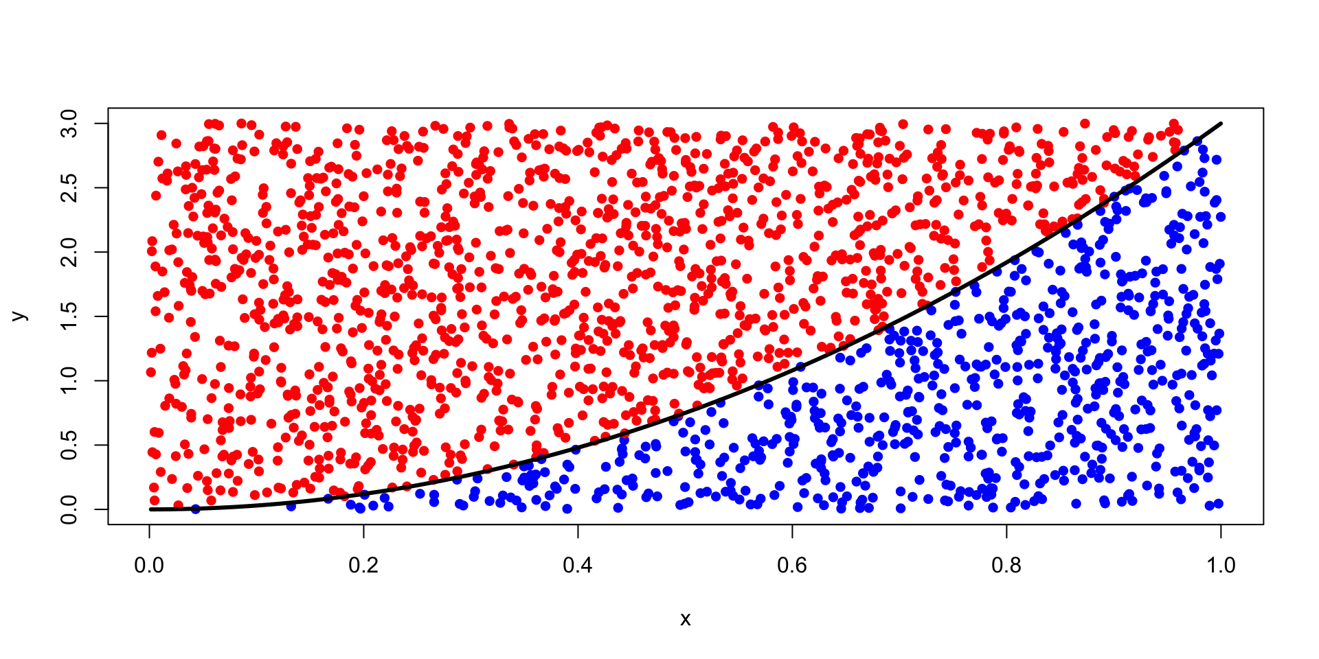
Why Does This Work?

  • Points are uniformly distributed in the rectangle.

  • Probability of acceptance:

    proportional to area under the curve.

👉 Accepted \(X\) values follow the target distribution.

# Visual points
x <- runif(2000)
y <- runif(2000, 0, 3)

plot(x, y, pch = 16, col = ifelse(y <= 3*x^2, "blue", "red"))
curve(3*x^2, add = TRUE, col = "black", lwd=3)
set.seed(1234)

n <- 10000

accepted <- numeric(0) # initialise numeric variables/vectors

while(length(accepted) < n){ # keep sampling until we have n accepted values
  x <- runif(1) # proposal: X ~ Uniform(0,1)
  y <- runif(1, 0, 3) # auxiliary variable: Y ~ Uniform(0, 3)
  
  if(y <= 3 * x^2){ # accept if point lies under the curve f(x)
    accepted <- c(accepted, x) # keep accepted x
  } # otherwise reject and try again
}

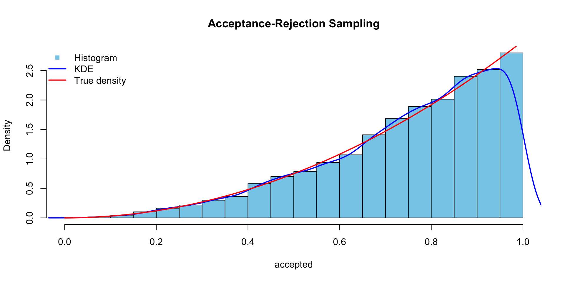
hist(accepted, prob = TRUE, col = "skyblue", main = "Acceptance-Rejection Sampling")
lines(density(accepted), col = "blue", lwd = 2) # Kernel Density Estimate (KDE)
curve(3 * x^2, col = "red", lwd = 2, add = TRUE) # True Density

legend("topright", legend = c("Histogram", "KDE", "True density"),
       col = c("skyblue", "blue", "red"),
       lwd = c(NA, 2, 2), pch = c(15, NA, NA), bty = "n")
  • The histogram matches the increasing shape of the target density, so larger values near 1 are more likely.
  • Small differences between bars and the curve are due to randomness and binning.

From Rectangles to General Envelopes

In the first example, we sampled uniformly from a rectangle and accepted points under the curve.

That works well when:

  • the support is simple
  • the density is bounded
  • a rectangle is easy to use

But many target densities are more complicated. Therefore, we need a more flexible idea.


Key Idea

Suppose we want to simulate from a target density \(f(x)\). Instead of sampling from a rectangle, we choose:

  • an easier density \(g(x)\)
  • a constant \(M > 0\)

such that

\[ \boxed{f(x) \le M g(x) \quad \forall x} \]

Then \(Mg(x)\) acts as an envelope over \(f(x).\)

👉 The closer \(Mg(x)\) is to \(f(x)\), the more efficient the method.

General Acceptance-Rejection Algorithm

To simulate \(X \sim f(x):\)

Generate a candidate
\(Y \sim g(x)\)
Generate
\(U \sim \text{Uniform}(0,1)\)
Accept \(Y\) if
\(U \le \dfrac{f(Y)}{M g(Y)}\)
Otherwise
reject \(Y\) and repeat
  • If the candidate \(Y\) is accepted, then we set \(X = Y\).
  • The accepted values follow the target density \(f(x)\).

Efficiency of the Method

The probability of acceptance is

\[ \frac{1}{M}. \]

  • smaller \(M\) \(\rightarrow\) higher acceptance rate
  • larger \(M\) \(\rightarrow\) more rejections

Choosing a Good Proposal Density

  • have the same support as \(f(x)\)
  • be easy to sample from
  • make \(M\) as small as possible
  • Uniform proposal on a bounded interval
  • Exponential proposal for right-skewed targets
  • Normal proposal for bell-shaped targets

Cubic Polynomial CDF Example (From Part 1)

The measurement error \(X\) (in mV) of a particular volt-meter has the following distribution:

\[ f(x) = \begin{cases} \dfrac{4-x^2}{9}, & \quad -1 \leq x \leq 2 \\ 0, & \text{otherwise.} \end{cases} \]

Simulate \(f(x)\) using acceptance-rejection method.

Step 0: Check whether \(f(x)\) is valid

\[ \int_{-1}^2 \frac{4-x^2}{9} \,dx = 1 \rightarrow \text{ valid PDF.} \]

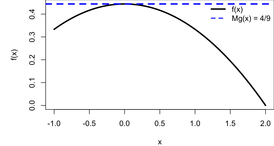
Step 1: Determine \(Mg(x); f(x) \leq Mg(x)\)

Because the support is bounded, the best first proposal is:

\[ g(x) = \text{Uniform}(-1, 2) = \frac{1}{3}, \quad -1 \leq x \leq 2. \]

Since \(g(x)=1/3\), this becomes

\[ \frac{4-x^2}{3} \leq M \]

Now on [-1, 2], the maximum of LHS occurs at \(x=0,\)

\[ \max_{-1\leq x \leq 2} \frac{4-x^2}{3} = \frac{4}{3} \]

Hence, we can choose

\[ M = \frac{4}{3} \quad \text{ with an acceptance rate of } \quad \frac{1}{M} = \frac{3}{4} = 75\% \]

This gives

\[ Mg(x) = \frac{4}{3} \cdot \frac{1}{3} = \frac{4}{9} \]

  • So the envelope is just a horizontal line at height 4/9.

Step 2: Determine the acceptance rule

The general rule is

\[ U \leq \frac{f(Y)}{Mg(Y)} \]

where \(Y\sim g\) and \(U \sim \text{Uniform}(0,1).\)

Substitute in, gives

\[ \frac{f(Y)}{Mg(Y)} = \frac{4-y^2}{4} \]

So accept \(Y\) if

\[ U \leq \frac{4-y^2}{4}. \]

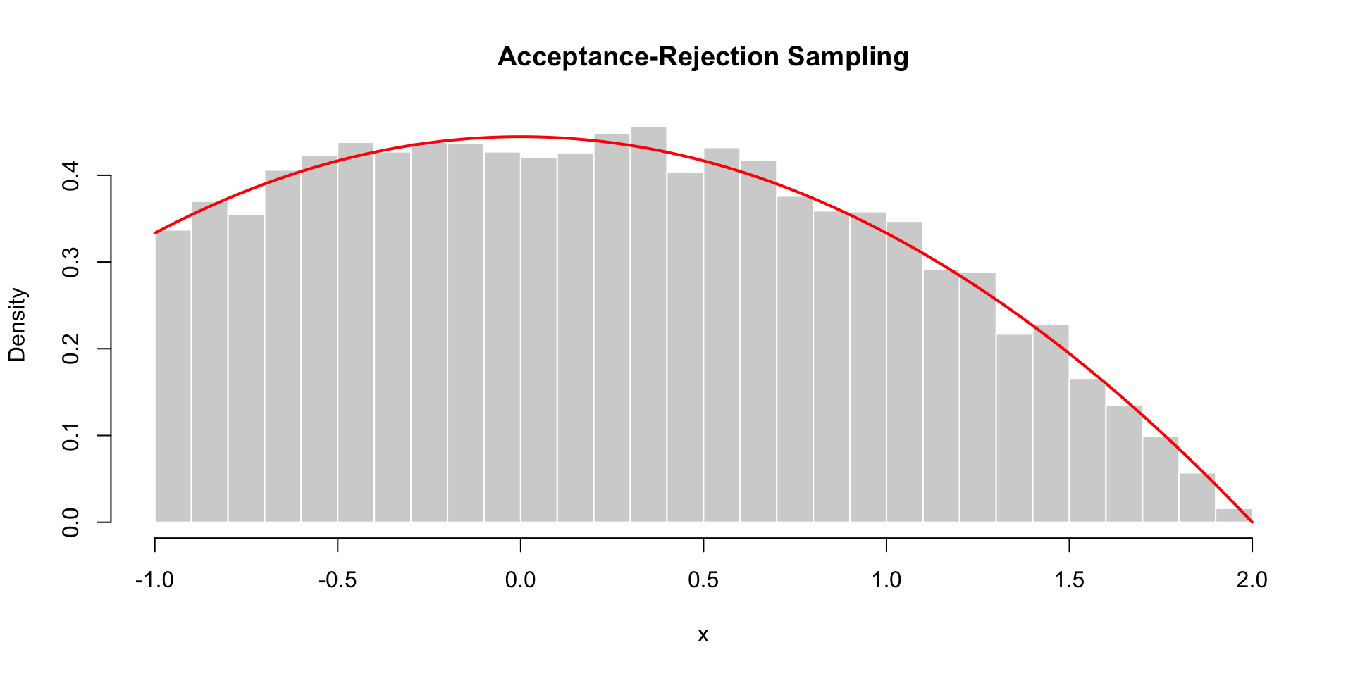
set.seed(1234)
n <- 10000
x <- numeric(0) # store accepted samples

while(length(x) < n){ # keep sampling until we have n accepted values
  y <- runif(n, min = -1, max = 2)   # proposal sample Y ~ g(x) ~ Uniform(-1, 2)
  u <- runif(n)                      # U ~ Uniform(0,1) for acceptance test
  accept <- u <= (4 - y^2)/4         # acceptance rule (returns TRUE/FALSE)
  x <- c(x, y[accept])               # keep accepted y
}

x <- x[1:n] # trim to exactly n samples
hist(x, prob = TRUE, breaks = 40,
     col = "lightgray", border = "white",
     main = "Acceptance-Rejection Sampling",
     xlab = "x")

curve((4 - x^2)/9, from = -1, to = 2,
      add = TRUE, col = "red", lwd = 2)

Normal-Cauchy Example

Generate the standard normal distribution using the standard Cauchy distribution

Recall the PDF of \(X \sim N(0, 1):\)

\[ f(x)=\frac{1}{\sqrt{2\pi}}\exp{\left(-\frac{x^2}{2}\right)}, \quad x \in \mathbb{R}. \]

The PDF of \(X \sim \text{Cauchy}:\)

\[ g(x) = \frac{1}{\pi(1+x^2)}, \quad x \in \mathbb{R}. \]

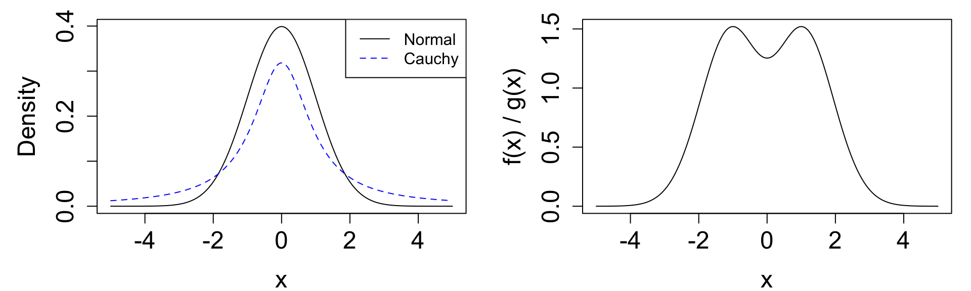
Let’s compare the distributions:

Code
x <- seq(-5, 5, length = 200)
dc <- dcauchy(x, location = 0, scale = 1)
dn <- dnorm(x, mean = 0, sd = 1)

par(mfrow=c(1,2), mar=c(4,5,1,1))
plot(x, dn, type="l", ylab="Density", cex.lab=1.5, cex.axis=1.5)
lines(x, dc, col="blue", lty=2)
legend("topright", col=c("black", "blue"), lty=c(1,2), legend =c("Normal", "Cauchy"))
plot(x, dn/dc, type="l", ylab="f(x) / g(x)", cex.lab=1.5, cex.axis=1.5)
  • From RHS, the standard cauchy distribution is wider but shorter than the standard normal distribution.
  • From LHS, the \(f(x)/g(x)\) ratio is maximised around 1.5.
Step 1: Find \(M\)

\[ \frac{f(x)}{g(x)} = \frac{1}{\sqrt{2\pi}}\exp{\left(-\frac{x^2}{2}\right)} \cdot \pi(1+x^2) = \frac{\pi}{\sqrt{2\pi}}(1+x^2)\exp{\left(-\frac{x^2}{2}\right)} \]

\[ \max_{-\infty < x < \infty}{(1+x^2)\exp{\left(-\frac{x^2}{2}\right)}} \]

Differentiate and set it equal to 0:

\[ \begin{aligned} \frac{d}{dx} \left(\frac{f(x)}{g(x)}\right) &= 2x\exp{\left(-\frac{x^2}{2}\right)} + (1+x^2)(-x)\exp{\left(-\frac{x^2}{2}\right)} \\ 0 &= \exp{\left(-\frac{x^2}{2}\right)} x (1-x^2) \end{aligned} \]

yields three critical points: \(x = 0, x = \pm 1.\)

  • From the ratio plot, we would expect the maximum to occur at \(x = \pm 1.\)

  • If this is not obvious, use the second derivative test to verify.

Substitute \(x= \pm 1\) into \(f(x)/g(x)\) yields

\[ M=2e^{-1/2}\sqrt{\frac{\pi}{2}}\approx 1.5203 \rightarrow \text{ with the acceptance probability of } 0.6577. \]

Step 2: Determine the acceptance rule

The general rule is

\[ U \leq \frac{f(Y)}{Mg(Y)} \]

where \(Y\sim g \sim \text{Cauchy}\) and \(U \sim \text{Uniform}(0,1).\)

Substitute in, gives the acceptance rule

\[ U \leq \frac{f(Y)}{Mg(Y)} = \frac{\sqrt{e}}{2} (1+y^2) \exp{\left(-\frac{y^2}{2}\right)} \]

set.seed(1234)
n <- 5000              # number of samples needed
M <- 2 * exp(-1/2) * sqrt(pi/2)   # exact M ≈ 1.5203
samples <- numeric(0)

while(length(samples) < n){
  y <- rcauchy(n) # propose from Cauchy
  u <- runif(n)   # uniform for acceptance
  f <- dnorm(y)   # target density
  g <- dcauchy(y) # proposal density
  
  accept <- u <= f / (M * g) # acceptance rule
  samples <- c(samples, y[accept])  # keep accepted values
}

samples <- samples[1:n] # trim to exactly n samples
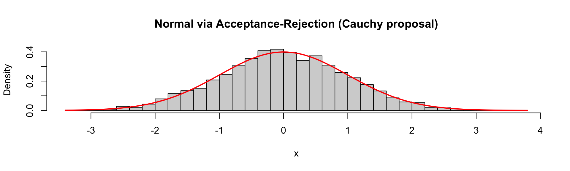
hist(samples, prob = TRUE, breaks = 40,
     col = "lightgray",
     main = "Normal via Acceptance-Rejection (Cauchy proposal)",
     xlab = "x")

curve(dnorm(x), add = TRUE, col = "red", lwd = 2)
set.seed(1234)
y <- rcauchy(5000); u <- runif(5000)
M <- 2 * exp(-1/2) * sqrt(pi/2)
accept <- u <= dnorm(y) / (M * dcauchy(y))
cat("The empirical acceptance rate is", mean(accept))
The empirical acceptance rate is 0.6578

Part 3: Precision of Simulation Result

Up until this point, we learned how to generate random variables using

  • known distributions
  • inverse transform
  • acceptance-rejection

We can now simulate almost any distribution.


How accurate are our simulation results?


  • If we simulate 1,000 samples… is that enough?
  • What about 10,000?
  • How close are we to the true value?


When we use these simulations to estimate quantities,

this is called Monte Carlo estimation.

Monte Carlo Estimation

Suppose we want to estimate:

\[ \mu = \mathbb{E}[X] \]

We simulate i.i.d random variables:

\[ X_1, X_2, \dots, X_n \]

and compute:

\[ \bar{X}_n = \frac{1}{n}\sum_{i=1}^n X_i, \]

where \(n\) is the number of simulated samples.


Key Result (CLT)

The CLT tells us about the distribution of \(\bar{X}_n\):

\[ \bar{X}_n \approx \mathcal{N}\left(\mu, \frac{\sigma^2}{n}\right) \]

based on the same \(n\) samples.


The CLT tells us that the error of Monte Carlo estimate is approximately Normally distributed for large \(n\), which allows us to construct confidence intervals and quantify simulation precision.

Monte Carlo Standard Error

The standard error measures simulation uncertainty:

\[ \text{SE}(\bar{X}_n) = \frac{\sigma}{\sqrt{n}} \]

In practice:

\[ \widehat{\text{SE}} = \frac{s}{\sqrt{n}} \]

where \(s\) is the sample standard deviation.

Interpretation: Larger \(n\) → smaller error, in which error decreases at rate \(1/\sqrt{n}.\)


set.seed(1234)

n <- 1000
x <- rexp(n, rate = 2)
x2 <- rexp(4*n, rate = 2)

mean(x); mean(x2)
[1] 0.5003067
[1] 0.5012854
sd(x)/sqrt(n); sd(x2)/sqrt(4*n)
[1] 0.01599075
[1] 0.007821783

Confidence Interval for the Mean

CI for sample mean is


\[ \bar{X}_n \pm z_{\alpha/2} \frac{s}{\sqrt{n}} \]

Confidence Level
\((1-\alpha)100\%\)
\(z_{\alpha/2}\)
90% \(1.645\)
95% \(1.960\)
99% \(1.645\)
Code
set.seed(1234)

n <- 1000
B <- 1000

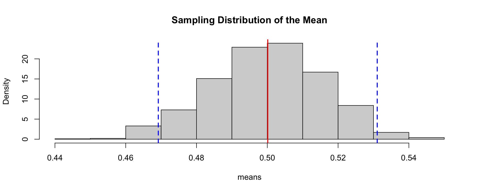
means <- replicate(B, mean(rexp(n, rate=2)))

hist(means, prob=TRUE, col="lightgray",
     main="Sampling Distribution of the Mean")

mean_est <- mean(means)
se <- sd(means)

abline(v = mean_est, col="red", lwd=2)
abline(v = mean_est + c(-1,1)*1.96*se,
       col="blue", lty=2, lwd=2)