STAT2005 Computer Simulation

Lecture 6 — Multivariate Simulation

Sam Wiwatanapataphee (275287a@curtin.edu.au)

2 Apr 2026

Goals today


  • Part 1: Transformation of Multiple RVs
    • Transformations of Two Random Variables
    • The Jacobian Formula


  • Part 2: Linear Transformations
    • Transformations of Random Vectors
    • Multivariate Normal Distribution
    • Cholesky


  • Part 3: Copulas
    • Gaussian Copula
    • Case Study: Portfolio risk simulation

Part 1: Transformation of Multiple RVs

Why Multivariate Simulation

In real-world problems, we rarely simulate a single variable in isolation.

Financial models → multiple asset returns

Example: Suppose you are managing a portfolio with three assets: Apple, Microsoft, and Tesla. Tech stocks usually move together, so we must simulate them jointly.

Reliability studies → lifetimes of related components

Example: Consider a car engine system with multiple components: battery, alternator, and starter motor. Each component has its own lifetime, but their lifetimes tend to fail together or degrade together (dependent).

Service systems → arrivals, service times, behaviour

Example: Consider a busy coffee shop during the morning rush. We need to simulate three interacting components: arrivals, service times, and customer behaviours.

Key Challenge

Simulating each variable separately is not enough.

We must also model dependence structure and joint behaviour

How Do We Do This?

We build from simple to powerful tools:

  • Transformations of two random variables
  • Linear transformations → correlation
  • Multivariate normal distribution
  • Cholesky decomposition → simulation
  • Copulas → flexible dependence modelling

Transformations of Two Random Variables

Suppose \((X, Y)\) has a known joint density \(f_{X,Y}(x,y)\), and we define a new pair:

\[ U = g_1(X, Y), \qquad V = g_2(X, Y). \]

Our goal is to find the joint density \(f_{U,V}(u,v).\)

If the transformation is one‑to‑one and differentiable, we can invert it:

\[ x = h_1(u,v), \qquad y = h_2(u,v), \]

and use the Jacobian determinant to adjust for how the transformation stretches or compresses area.

If the transformation is smooth and invertible, then

\[ \boxed{f_{U,V}(u,v) = f_{X,Y}(h_1(u,v),\, h_2(u,v)) \left| \det J \right|} \]

where

\[ J = \begin{pmatrix} \dfrac{\partial x}{\partial u} & \dfrac{\partial x}{\partial v} \\ \dfrac{\partial y}{\partial u} & \dfrac{\partial y}{\partial v} \end{pmatrix} \]

is the Jacobian matrix of the inverse transformation.

The \(|\det J|\) measures how the transformation changes area, ensuring that total probability remains 1.

Example 1: Sums and Differences

Let \((X,Y)\) have joint density \(f_{X,Y}(x,y)\). Define

\[ U = X + Y, \qquad V = X - Y. \]

This transformation is linear and invertible, and the Jacobian is constant.

Step 1: Invert the transformation

Solve for \(X, Y\) in terms of \(U, V\):

\[ X = \dfrac{U + V}{2}, \qquad Y = \dfrac{U - V}{2}. \]

So

\[ x = h_1(u,v) = \dfrac{u+v}{2}, \quad y = h_2(u,v) = \dfrac{u-v}{2}. \]

Step 2: Compute the Jacobian

\[ J = \begin{pmatrix} \dfrac{\partial x}{\partial u} & \dfrac{\partial x}{\partial v} \\ \dfrac{\partial y}{\partial u} & \dfrac{\partial y}{\partial v} \end{pmatrix} = \begin{pmatrix} \dfrac{1}{2} & \dfrac{1}{2} \\ \dfrac{1}{2} & -\dfrac{1}{2} \end{pmatrix}. \]

Then

\[ \det J = \dfrac{1}{2}\cdot\left(-\dfrac{1}{2}\right) - \dfrac{1}{2}\cdot\dfrac{1}{2} = -\dfrac{1}{4} - \dfrac{1}{4} = -\dfrac{1}{2}, \]

so

\[ |\det J| = \dfrac{1}{2}. \]

Step 3: Write the joint density of \((U, V)\)

\[ f_{U,V}(u,v) = f_{X,Y}\!\left(\dfrac{u+v}{2}, \dfrac{u-v}{2}\right)\cdot \dfrac{1}{2}. \]

Code
set.seed(1234)

n <- 5000
X <- rnorm(n)
Y <- rnorm(n)

U <- X + Y
V <- X - Y

par(mfrow = c(1, 2))

plot(X, Y, pch = 16, cex = 0.4, col = "steelblue",
     main = "Original (X, Y)",
     xlab = "X", ylab = "Y")

plot(U, V, pch = 16, cex = 0.4, col = "tomato",
     main = "Transformed (U = X+Y, V = X-Y)",
     xlab = "U", ylab = "V")

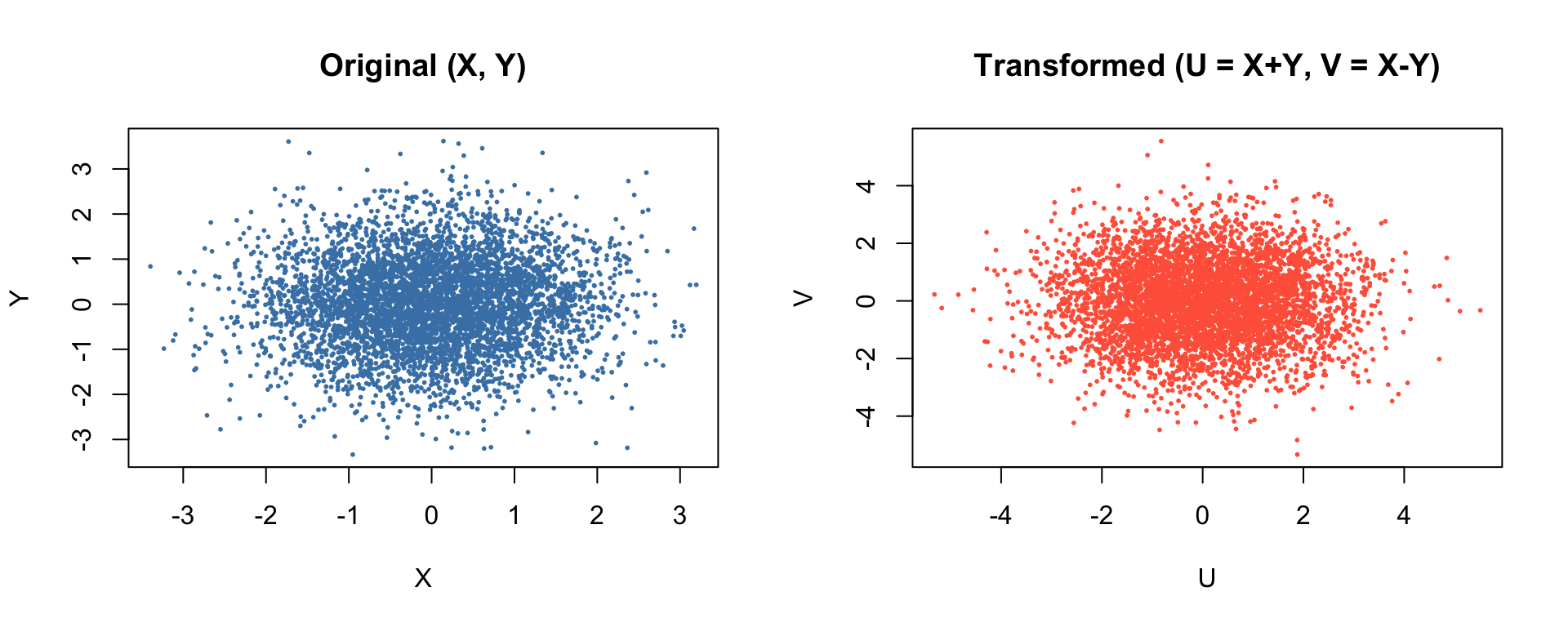
  • \((X,Y)\) is a round cloud (independent normals).
  • \((U,V)\) becomes an axis‑aligned ellipse — the transformation stretches and rotates the cloud.
  • This visually confirms the Jacobian‑based derivation.

Example 2: Polar Coordinates

Let \((X, Y)\) have joint density \(f_{X,Y}(x,y)\). Define

\[ U = R = \sqrt{X^2 + Y^2}, \qquad V = \Theta = \arctan(Y/X). \]

The Jacobian determinant is \(r\), which explains why polar integrals include the factor \(r\).

We want \(f_{R,\Theta}(r,\theta)\).

Step 1: Invert the transformation

The inverse map is the usual polar–Cartesian relation:

\[ X = r\cos\theta, \qquad Y = r\sin\theta. \]

So

\[ x = h_1(r,\theta) = r\cos\theta, \quad y = h_2(r,\theta) = r\sin\theta. \]

Step 2: Compute the Jacobian

\[ J = \begin{pmatrix} \dfrac{\partial x}{\partial r} & \dfrac{\partial x}{\partial \theta} \\ \dfrac{\partial y}{\partial r} & \dfrac{\partial y}{\partial \theta} \end{pmatrix} = \begin{pmatrix} \cos\theta & -r\sin\theta \\ \sin\theta & r\cos\theta \end{pmatrix}. \]

Then

\[ \det J = \cos\theta \cdot r\cos\theta - (-r\sin\theta)\cdot\sin\theta = r(\cos^2\theta + \sin^2\theta) = r. \]

So

\[ |\det J| = r. \]

Step 3: Joint density of \((R,\Theta)\)

\[ f_{R,\Theta}(r,\theta) = f_{X,Y}(r\cos\theta, r\sin\theta)\cdot r. \]

Code
set.seed(1234)

n <- 5000
X <- rnorm(n)
Y <- rnorm(n)

R <- sqrt(X^2 + Y^2)
Theta <- atan2(Y, X)

par(mfrow = c(1, 2))

hist(R, breaks = 40, freq = FALSE, col = "lightgray",
     main = "Distribution of R",
     xlab = "R")
curve(dchisq(x^2, df = 2) * 2*x, add = TRUE, col = "darkgreen", lwd = 2)

hist(Theta, breaks = 40, freq = FALSE, col = "lightblue",
     main = "Distribution of Theta",
     xlab = expression(theta))

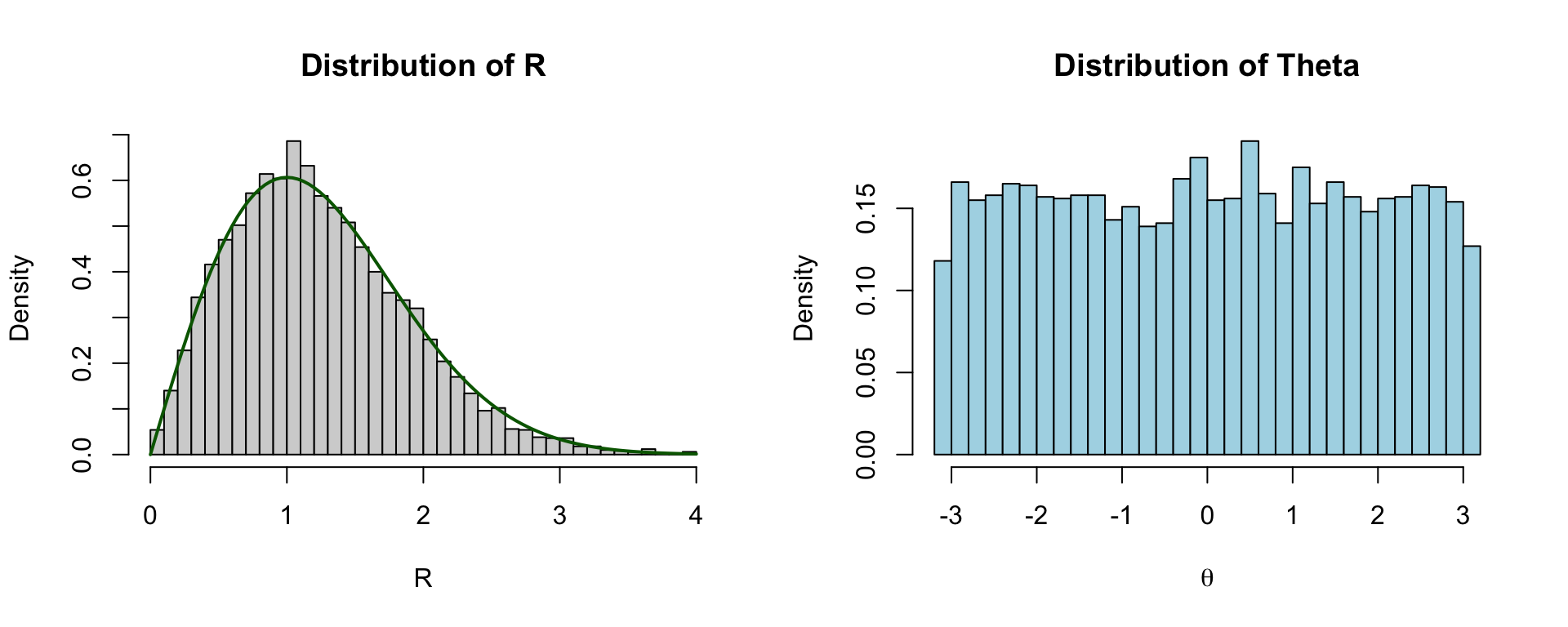
  • R follows the Rayleigh distribution (equivalently, \(R^2\sim \chi_2^2\)).
  • \(\Theta\) is uniform on \([-\pi ,\pi ]\).
Code
par(mfrow = c(1, 3))

plot(X, Y, pch = 16, cex = 0.4, col = "steelblue",
     main = "Original (X, Y)",
     xlab = "X", ylab = "Y")

plot(R, Theta, pch = 16, cex = 0.4, col = "green",
     main = "Transformed (R, Theta)",
     xlab = "R", ylab = "Theta")

plot(R*cos(Theta), R*sin(Theta), pch = 16, cex = 0.4, col = "tomato",
     main = "Back to Cartesian via Polar",
     xlab = "Rcos(theta)", ylab = "Rsin(theta)")
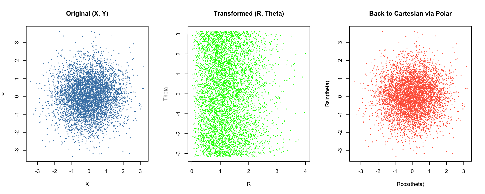
  • Original \((X, Y)\) shows a circular cloud centred at the origin.
  • Transformed \((R, \Theta)\) shows a rectangular cloud with horizontal axis \(R \ge 0\) and vertical axis \(\Theta \in [-\pi, \pi].\)
  • Revert back to cartesian via polar using \((X,Y) = (Rcos(\Theta), Rsin(\Theta))\), then the same circular cloud reappears.

Example 3: Linear Transformations

Let \((X, Y)\) have joint density \(f_{X,Y}(x,y)\), and let

\[ \begin{pmatrix} U \\ V \end{pmatrix} = A \begin{pmatrix} X \\ Y \end{pmatrix}, \quad A = \begin{pmatrix} a & b \\ c & d \end{pmatrix}, \]

with \(\det A \neq 0\). Then the Jacobian determinant is simply \(|\det A|\).

This case is especially important for the multivariate normal distribution, where linear transformations create covariance structures. The correlated‑normal simulation you used earlier is a special case of this idea.

Step 1: Invert the transformation

Because \(\det A \neq 0\), \(A\) is invertible:

\[ \begin{pmatrix} X \\ Y \end{pmatrix} = A^{-1} \begin{pmatrix} U \\ V \end{pmatrix}. \]

\[ A^{-1} = \frac{1}{ad - bc} \begin{pmatrix} d & -b \\ -c & a \end{pmatrix}. \]

So

\[ x = h_1(u,v), \quad y = h_2(u,v) \]

are linear functions of \((u,v)\).

Step 2: Jacobian of the inverse

For a linear map, the Jacobian matrix of the inverse is just \(A^{-1}\), so

\[ |\det J| = |\det A^{-1}| = \frac{1}{|\det A|}. \]

Step 3: Joint density of \((U,V)\)

\[ f_{U,V}(u,v) = f_{X,Y}\big(h_1(u,v), h_2(u,v)\big)\cdot \frac{1}{|\det A|}. \]

Code
set.seed(1234)

n <- 5000
X <- rnorm(n)
Y <- rnorm(n)

A <- matrix(c(1, 0.8,
              0.2, 1), nrow = 2, byrow = TRUE)

UV <- A %*% rbind(X, Y)
U <- UV[1, ]
V <- UV[2, ]

par(mfrow = c(1, 2))

plot(X, Y, pch = 16, cex = 0.4, col = "gray40",
     main = "Original (X, Y)",
     xlab = "X", ylab = "Y")

plot(U, V, pch = 16, cex = 0.4, col = "firebrick",
     main = "Transformed (U, V) = A(X, Y)",
     xlab = "U", ylab = "V")

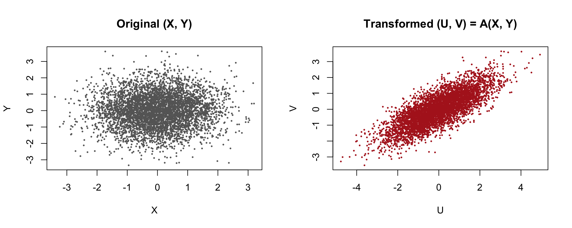
  • The original cloud is round (independent normals).
  • The transformed cloud becomes tilted and stretched, showing induced correlation.

Part 2: Linear Trasformations and the Multivariate Normal

Why Linear Transformation

Linear transformations are central to probability and statistics, especially for multivariate normal distributions.

A key idea:

  • start with independent standard normals
  • apply a matrix transformation
  • create correlation and covariance structure

This lets us construct any multivariate normal distribution from a standard one.

Why This Matters

Linear transformations underpin:

  • simulation of correlated variables
  • regression and linear models
  • principal component analysis (PCA)
  • Bayesian multivariate priors
  • many other multivariate methods

This topic is the bridge between:

probability theory and practical statistical modelling

Linear Transformations of Random Vectors

Let

\[ \mathbf{X} = (X_1, X_2, \dots, X_k)^\top \]

be a random vector, and let \(A\) be a fixed \(m \times k\) matrix.

A linear transformation of \(\mathbf{X}\) is

\[ \boxed{\mathbf{Y} = A\mathbf{X} + \mathbf{b}} \]

where \(\mathbf{b}\) is a constant vector.

This transformation:

  • rotates, stretches, or compresses the space,
  • shifts the mean by \(\mathbf{b}\),
  • and reshapes the covariance structure through the matrix \(A\).

The Multivariate Normal Distribution

Why Multivariate Normal (MVN)?

It is the only multivariate distribution that is stable under linear transformation and fully characterised by mean + covariance.

That makes it mathematically tractable, computationally efficient, and an ideal building block for simulating dependence.

A random vector \(\mathbf{X}\) is MVN:

\[ \mathbf{X} \sim N(\boldsymbol{\mu}, \Sigma), \]

  • \(\boldsymbol{\mu}\) is the mean vector,
  • \(\Sigma\) is the covariance matrix (symmetric and positive‑definite).

\[ f_{\mathbf{X}}(\mathbf{x}) = \frac{1}{(2\pi)^{k/2} |\Sigma|^{1/2}} \exp\!\left( -\frac{1}{2}(\mathbf{x}-\boldsymbol{\mu})^\top \Sigma^{-1}(\mathbf{x}-\boldsymbol{\mu}) \right). \]

\[ \mathbf{X} \sim N(\boldsymbol{\mu}, \Sigma) \quad \Longrightarrow \quad A\mathbf{X} + \mathbf{b} \sim N(A\boldsymbol{\mu} + \mathbf{b},\; A\Sigma A^\top). \]

This means:

  • linear transformations of normals are still normal (preserve normality),
  • the mean transforms linearly,
  • the covariance transforms quadratically.

Example 4: Linear Transformation of a Bivariate Normal

Simulate \(\mathbf{X}\sim N(\mu ,\Sigma )\) with mean vector and covariance matrix:

\[ \mu = (1,2)^{\top}, \qquad \Sigma =\left( \begin{matrix}4&1\\ 1&1\end{matrix}\right). \]

The entries encode \(\text{Var}(X_1) = 4\), \(\text{Var}(X_2) = 1\) and \(\text{Cov}(X_1,X_2) = 1\).

Then, apply \(\mathbf{Y}=A\mathbf{X}+b\) with

\[ A =\left( \begin{matrix}1&0\\ -1&2\end{matrix}\right), \qquad b = (0, 1)^{\top} \]

Code
set.seed(1234)

library(MASS)

# Original distribution
mu  <- c(1, 2)
Sigma <- matrix(c(4, 1,
                  1, 1), 2, 2)

n <- 5000
X <- mvrnorm(n, mu = mu, Sigma = Sigma)

# Linear transformation
A <- matrix(c(1, 0,
             -1, 2), 2, 2)
b <- c(0, 1)

# Matrix algebra
Y <- t(A %*% t(X)) + matrix(b, n, 2, byrow = TRUE)

par(mfrow = c(1, 2), mar = c(4,4,1,1))

plot(X[,1], X[,2], pch = 16, cex = 0.4, col = "steelblue",
     main = "Original X ~ N(mu, Sigma)",
     xlab = "X1", ylab = "X2")

plot(Y[,1], Y[,2], pch = 16, cex = 0.4, col = "tomato",
     main = "Transformed Y = A X + b",
     xlab = "Y1", ylab = "Y2")
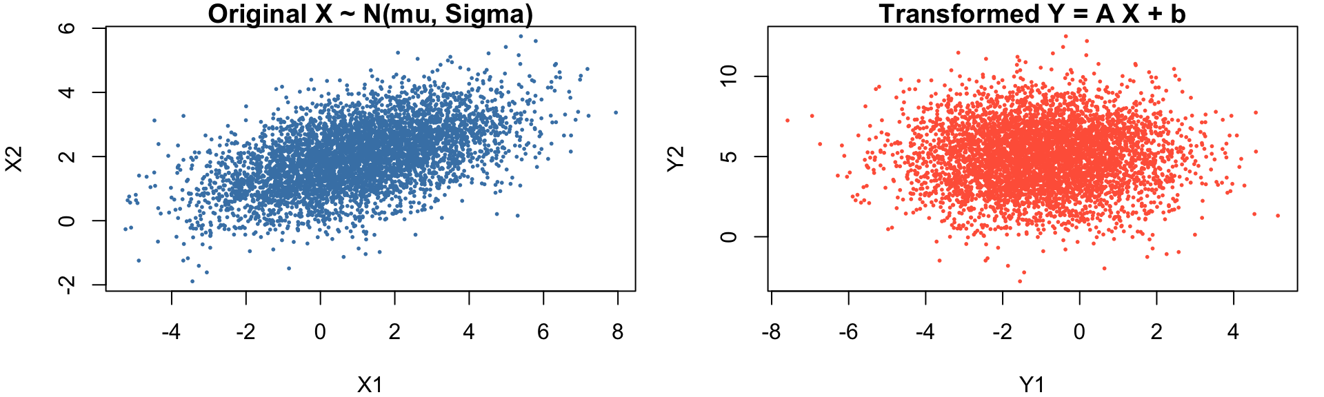
  • The original cloud has a certain tilt and spread.
  • The transformed cloud is rotated and stretched exactly as predicted by \(A\Sigma A^{\top }\).

Constructing a Multivariate Normal via Cholesky

  • To simulate correlated variables, we need a way to impose a given covariance structure on independent normals.
  • The Cholesky decomposition provides a simple and efficient solution.
  • It transforms standard normal variables into correlated ones using a matrix factorisation of the covariance matrix.
  • This generalises the familiar two-dimensional construction to higher dimensions.

If \(\Sigma\) is a covariance matrix, we can write:

\[ \Sigma = LL^\top, \]

where \(L\) is the Cholesky factor (lower triangular).

If \(\mathbf{Z} \sim N(\mathbf{0}, I)\), then

\[ \mathbf{X} = L\mathbf{Z} + \boldsymbol{\mu} \]

has distribution \(N(\boldsymbol{\mu}, \Sigma)\).

This generalises earlier 2D construction:

\[ X = \rho Z_1 + \sqrt{1-\rho^2}\, Z_2, \]

which is exactly the Cholesky factor of \(\begin{pmatrix}1 & \rho \\ \rho & 1\end{pmatrix}\).

Example 5: Constructing Correlated Normals via Cholesky

Define the covariance matrix

\[\Sigma =\left( \begin{matrix}1&\rho \\ \rho &1\end{matrix}\right) =\left( \begin{matrix}1&0.8\\ 0.8&1\end{matrix}\right).\]

Code
set.seed(1234)

n <- 5000
rho <- 0.8

# Covariance matrix
Sigma <- matrix(c(1, rho,
                  rho, 1), 2, 2)

# Cholesky factor: L^T L (upper triangular)
L <- chol(Sigma)

# Generate 2n independent N(0,1) values
Z <- matrix(rnorm(2*n), n, 2)

# Construct X = Z L^T (linear transformation)
X <- Z %*% L

par(mfrow = c(1, 2), mar = c(4,4,1,1))

plot(Z[,1], Z[,2], pch = 16, cex = 0.4, col = "gray60",
     main = "Z ~ N(0, I)",
     xlab = "Z1", ylab = "Z2")

plot(X[,1], X[,2], pch = 16, cex = 0.4, col = "firebrick",
     main = "X = Z L^T (Correlated Normals)",
     xlab = "X1", ylab = "X2")

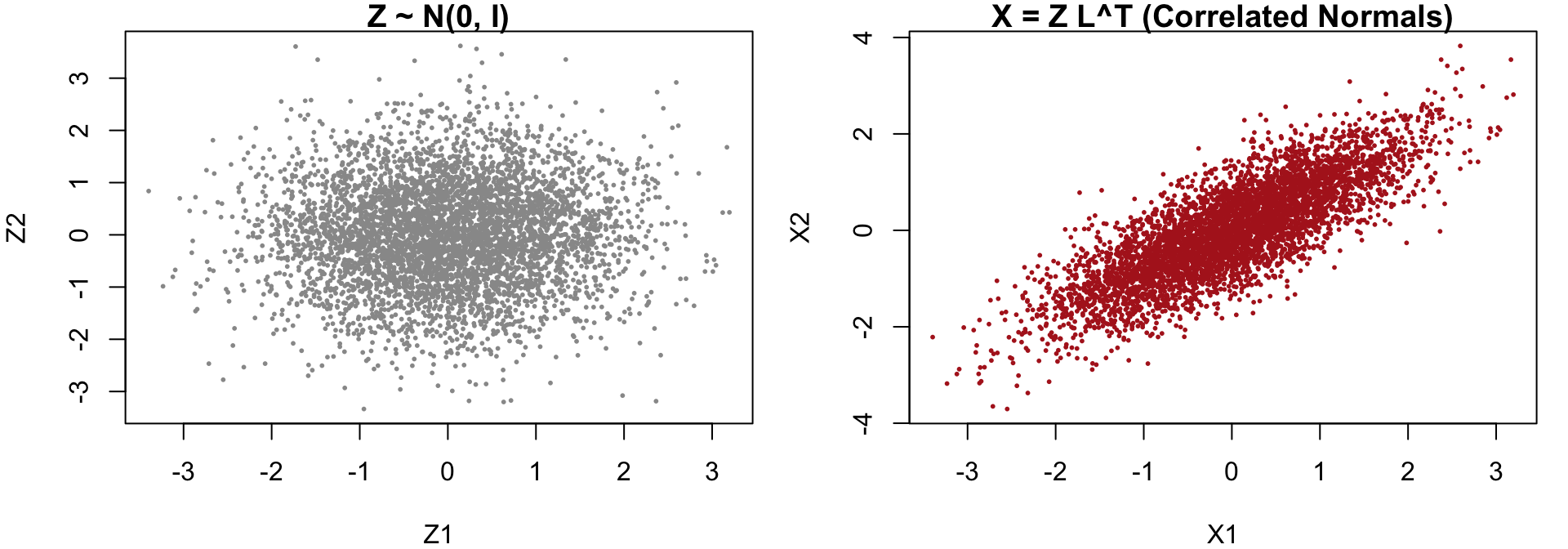
  • \(Z\) is a round cloud (independent normals).
  • \(X\) becomes a tilted ellipse with correlation \(\rho =0.8\).
  • This is how Cholesky induces covariance.

Example 6: General k‑Dimensional Construction

Simulate \(\mathbf{X}\sim N(\mu ,\Sigma )\) using Cholesky. Define a mean vector and a covariance matrix:

\[ \mu =(0,\; 1,\; 2)^{\top }, \qquad \Sigma =\left( \begin{matrix}1&0.5&0.2\\ 0.5&2&0.3\\ 0.2&0.3&1\end{matrix}\right). \]

set.seed(1234)
mu <- c(0, 1, 2)
Sigma <- matrix(c(1, 0.5, 0.2,
                  0.5, 2, 0.3,
                  0.2, 0.3, 1), 3, 3)

n <- 5000
L <- chol(Sigma) # Cholesky factor L^T
Z <- matrix(rnorm(3*n), n, 3) # Standard normals

# Construct X = Z L^T + mu
X <- Z %*% L + matrix(mu, n, 3, byrow = TRUE)

round(cov(X), 2) # sample covariance
     [,1] [,2] [,3]
[1,] 0.98 0.54 0.21
[2,] 0.54 1.98 0.31
[3,] 0.21 0.31 1.00
  • The sample covariance of \(X\) matches \(\Sigma\), suggesting the construction works in any dimension.
Code
# 3D scatterplot
library(scatterplot3d)

scatterplot3d(X[,1], X[,2], X[,3],
              pch = 16, cex.symbols = 0.4,
              color = "steelblue",
              main = "3D Scatterplot of Multivariate Normal Sample",
              xlab = "X1", ylab = "X2", zlab = "X3")
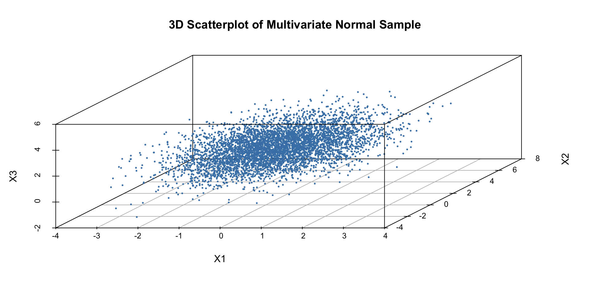
  • A 3D elliptical cloud whose shape reflects the covariance matrix.
  • The cloud is tilted and stretched in directions determined by \(\Sigma\).
  • This visually reinforces the idea that \(X=LZ+\mu\).

Part 3: Copulas

Why Copulas

So far, we have constructed dependence using linear transformations and Cholesky decomposition.

This approach is powerful, but it has an important limitation:

It ties dependence to normality.

In many real-world applications (finance, insurance, environmental modelling), dependence can be:

  • non-linear,
  • asymmetric,
  • or stronger in extremes (tail dependence).

To model such behaviour, we need a more flexible framework.

This leads to the idea of copulas.


A copula is a function that allows us to construct a joint distribution by combining:

  • marginal distributions, and
  • a dependence structure.

Copula

Key Idea

Any joint distribution can be decomposed as:

\[ F_{X,Y}(x,y) = C\big(F_X(x), F_Y(y)\big), \]

where:

  • \(F_X, F_Y\) are marginal CDFs,
  • \(C(u,v)\) is a copula.

This result is known as Sklar’s Theorem.

Interpretation

  • Marginals describe individual behaviour.
  • The copula describes dependence.

Why Copulas Matter in Simulation

Copulas allow us to:

  • simulate dependence without assuming normality,
  • combine any marginal distributions (e.g., Normal + Exponential),
  • model tail dependence (important in risk modelling),
  • separate modelling into marginals (easy) or dependence (flexible).

Gaussian Copula

The most commonly used copula in simulation is the Gaussian copula.


Simulation Algorithm

  1. Choose:
    • marginal distributions \(F_X, F_Y\),
    • correlation parameter \(\rho\)
  1. Construct covariance matrix \(\hspace{7em} \Sigma =\begin{pmatrix}1 & \rho \\\rho & 1 \end{pmatrix}\)
  1. Generate \(\hspace{13em} (Z_1, Z_2) \sim N(0, \Sigma)\)
  1. Transform \(\hspace{14em} U_i = \Phi(Z_i)\)
  1. Apply inverse CDF \(\hspace{7em} X = F_X^{-1}(U_1), \quad Y = F_Y^{-1}(U_2)\)

Example 7: Normal–Exponential Dependence

Simulate \(X \sim N(0,1)\) and \(Y \sim \text{Exp}(1)\) with dependence \(\rho = 0.7\)

Code
set.seed(1234)

library(MASS)

n <- 5000
rho <- 0.7

# Step 1: correlated normals
Sigma <- matrix(c(1, rho,
                  rho, 1), 2, 2)

Z <- mvrnorm(n, mu = c(0,0), Sigma = Sigma)

# Step 2: convert to uniforms
U <- pnorm(Z)

# Step 3: apply inverse CDFs
X <- qnorm(U[,1])      # Normal
Y <- qexp(U[,2])       # Exponential

plot(X, Y, pch = 16, cex = 0.4, col = "steelblue",
     main = "Gaussian Copula (Normal + Exponential)",
     xlab = "X ~ N(0,1)", ylab = "Y ~ Exp(1)")
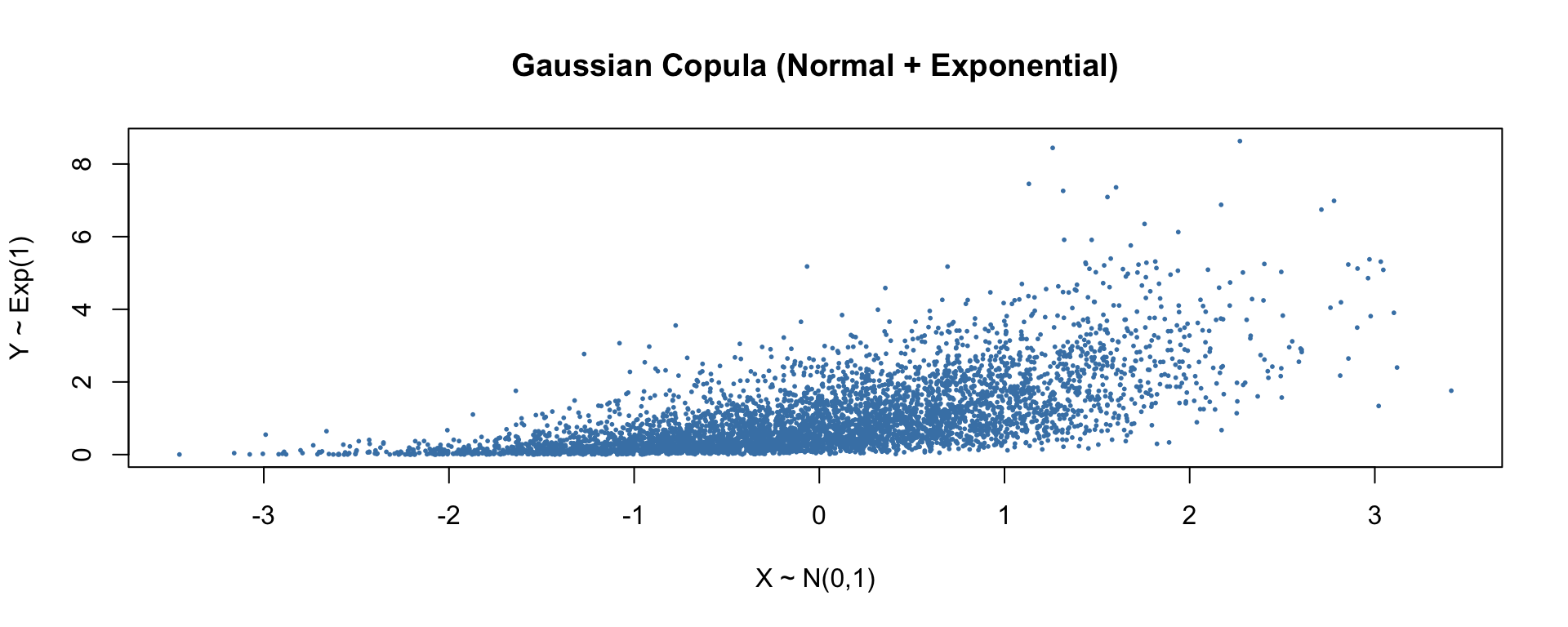
  • Marginals are preserved exactly,
  • Dependence is induced via the copula,
  • The shape is not elliptical (unlike MVN).

Limitations

The Gaussian is weak in modelling extreme co-movements. Alternatively, we can use t-copula to capture tail dependence, Clayton copula to capture lower tail dependence, or Gumbel copula to capture upper tail dependence.

Simulation of Dependent Variables (Summary)

Linear Transformation Copula-Based Simulation
Use \(X=LZ+\mu\) \(U_i = \Phi(Z_i), \quad X_i = F_i^{-1}(U_i)\)
Works for Normal only Any marginals
Dependence Linear Flexible
Pros Simple and efficient Very flexible, realistic modelling
Cons Limited flexibility Slightly more complex
Use case Statistics, regression Finance, risk, insurance


General Algorithm

  1. Specify marginals \(F_1, \dots, F_k\)
  2. Choose dependence structure: covariance matrix (MVN) or copula
  3. Generate base variables: \(Z \sim N(0,I)\)
  4. Induce dependence via \(LZ\) (Cholesky) or copula
  5. Transform to desired marginals

📈 Case Study: Portfolio Risk Simulation

📈 Case Study: Portfolio Risk Simulation

In this example, we study the distribution of returns, which describes how much an asset or portfolio gains or loses over time (e.g., daily returns). Understanding this distribution helps answer questions such as:

  • How large can losses be?
  • How likely are extreme events?
  • How does dependence between assets affect risk?

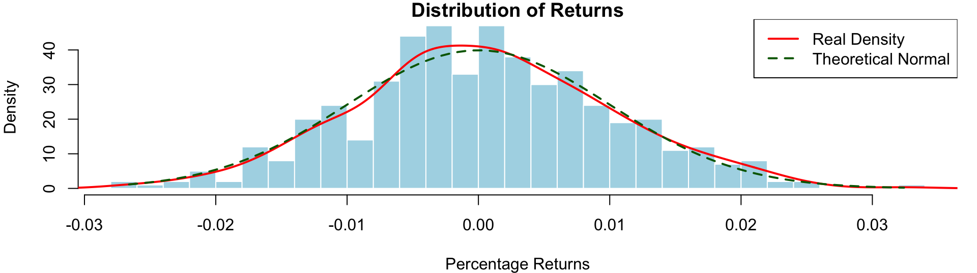
Financial theory assumes that returns follow a normal (Gaussian) or lognormal distribution, which means:

  • most outcomes are close to the average (symmetric around the mean),
  • extreme gains or losses are rare,
  • dependence between assets is captured using correlation.

In practice, returns often behave differently:

  • Fat tails: Extreme events occur more often than predicted by a normal distribution.
  • High peaks (leptokurtosis): Returns may be more concentrated around the mean.
  • Skewness: Distributions may be asymmetric, with markets reacting differently to positive versus negative events (overreaction or underreaction).
  • Dependency: Dependence between assets can become stronger during extreme events.

This means simple normal models may underestimate risk, especially for large losses.

Problem Statement

A financial analyst wants to model the joint daily returns of two assets in a portfolio, Asset A and Asset B, with equal weights of 50%.

The analyst wants to estimate:

  • the mean and standard deviation of the portfolio return
  • the 1% and 5% Value-at-Risk (VAR), and
  • the probability of a large one-day portfolio loss.

Since the asset returns are dependent, simulating each asset separately would underestimate the risk of simultaneous losses.

Therefore, the analyst considers three modelling approaches:

  • a multivariate normal model as a baseline for correlated returns,
  • a copula-based model to allow more flexible marginal distributions and dependence, especially under extreme market conditions, and
  • an independent model as a benchmark.

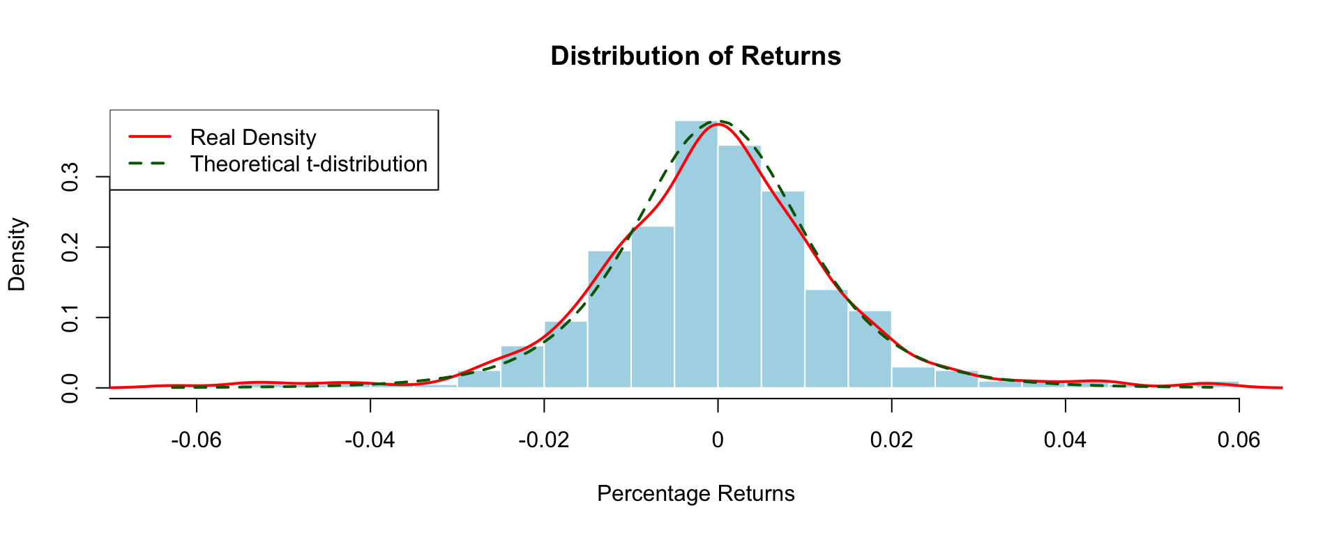
The analyst then conduct data analysis to understand the distribution of returns for Asset A and Asset B.

Multivariate Normal Model

The portfolio weights are

\[ w_1 = 0.5, \qquad w_2 = 0.5, \]

so the portfolio return is

\[ R_p = 0.5R_1 + 0.5R_2. \]

Based on the data analysis, the analyst assumes:

  • \(R_1\) has a Normal marginal distribution, \(R_1 \sim N(0.0005, 0.015^2)\).
  • \(R_2\) has a Normal marginal distribution, \(R_2 \sim N(0.0008, 0.02^2)\).
  • Dependence is introduced via a covariance matrix with correlation \(\rho = 0.6\).
library(MASS)
set.seed(1234)
n <- 10000
rho <- 0.6 # correlation
w <- c(0.5, 0.5) # Portfolio weights
mu <- c(0.0005, 0.0008) # Mean vector (daily returns)
sd1 <- 0.015 # standard deviation of R1
sd2 <- 0.02  # standard deviation of R2
Sigma <- matrix(c(sd1^2, rho*sd1*sd2,
                  rho*sd1*sd2, sd2^2), 2, 2) # Covariance matrix
R_gauss <- mvrnorm(n, mu = mu, Sigma = Sigma) # Simulate correlated normal returns
port_gauss <- R_gauss %*% w # Portfolio return
Code
risk_summary <- c(
  Mean = mean(port_gauss), # mean of portfolio return
  SD = sd(port_gauss),     # standard devation of portfolio return
  VaR_5 = quantile(port_gauss, 0.05), # 5% Value-at-Risk
  VaR_1 = quantile(port_gauss, 0.01), # 1% Value-at-Risk
  Prob_Loss_gt_3pct = mean(port_gauss < -0.03) # probability of losing more than 3% in one day
)

library(knitr)
kable(round(risk_summary, 4))
x
Mean 0.0008
SD 0.0155
VaR_5.5% -0.0248
VaR_1.1% -0.0352
Prob_Loss_gt_3pct 0.0232
Code
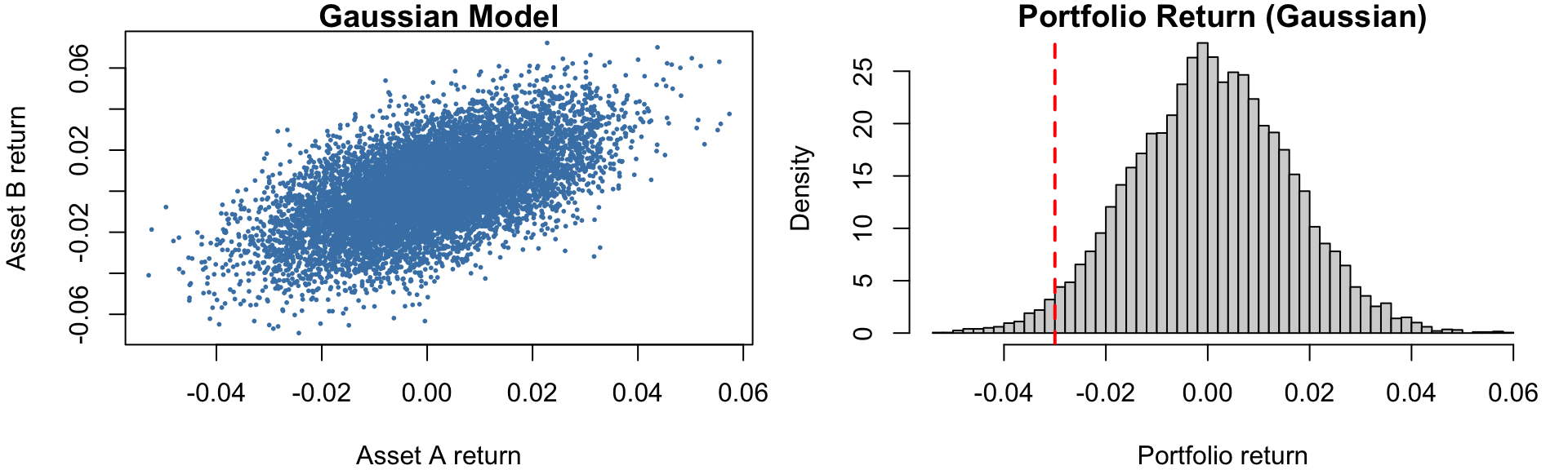
par(mfrow = c(1, 2), mar = c(4,4,1,1))

plot(R_gauss[,1], R_gauss[,2],
     pch = 16, cex = 0.4, col = "steelblue",
     main = "Gaussian Model",
     xlab = "Asset A return", ylab = "Asset B return")

hist(port_gauss, breaks = 40, freq = FALSE, col = "lightgray",
     main = "Portfolio Return (Gaussian)",
     xlab = "Portfolio return")
abline(v = -0.03, col = "red", lwd = 2, lty = 2)

Copula-based Model

The portfolio weights and portfolio return are

\[ w_1 = 0.5, \qquad w_2 = 0.5, \qquad R_p = 0.5R_1 + 0.5R_2. \]

Based on the data analysis, the analyst assumes:

  • \(R_1\) has a Normal marginal distribution, \(R_1 \sim N(0.0005, 0.015^2)\).
  • \(R_2\) has a heavier-tailed \(t\) marginal distribution with 4 degrees of freedom, rescaled to have approximately standard deviation \(0.02\).
  • Dependence is introduced using a Gaussian copula with correlation \(\rho = 0.6\).
set.seed(1234)
n <- 10000
rho <- 0.6  # Correlation
Sigma_cop <- matrix(c(1, rho, rho, 1), 2, 2)
Z <- mvrnorm(n, mu = c(0, 0), Sigma = Sigma_cop) 
U <- pnorm(Z) # Convert to Uniform

# Asset A: Normal marginal
X1 <- qnorm(U[,1], mean = 0.0005, sd = 0.015)

# Asset B: heavy-tailed t marginal
# Standard t(df=4) has variance df/(df-2) = 2, so divide by sqrt(2)
# to approximately standardise before scaling
X2 <- 0.0008 + 0.02 * (qt(U[,2], df = 4) / sqrt(2))

R_copula <- cbind(X1, X2)
port_copula <- R_copula %*% w # Portfolio return
Code
risk_summary2 <- c(
  Mean = mean(port_copula), # mean of portfolio return
  SD = sd(port_copula),     # standard devation of portfolio return
  VaR_5 = quantile(port_copula, 0.05), # 5% Value-at-Risk
  VaR_1 = quantile(port_copula, 0.01), # 1% Value-at-Risk
  Prob_Loss_gt_3pct = mean(port_copula < -0.03) # probability of losing more than 3% in one day
)

library(knitr)
kable(round(risk_summary2, 4))
x
Mean 0.0007
SD 0.0153
VaR_5.5% -0.0238
VaR_1.1% -0.0378
Prob_Loss_gt_3pct 0.0235
Code
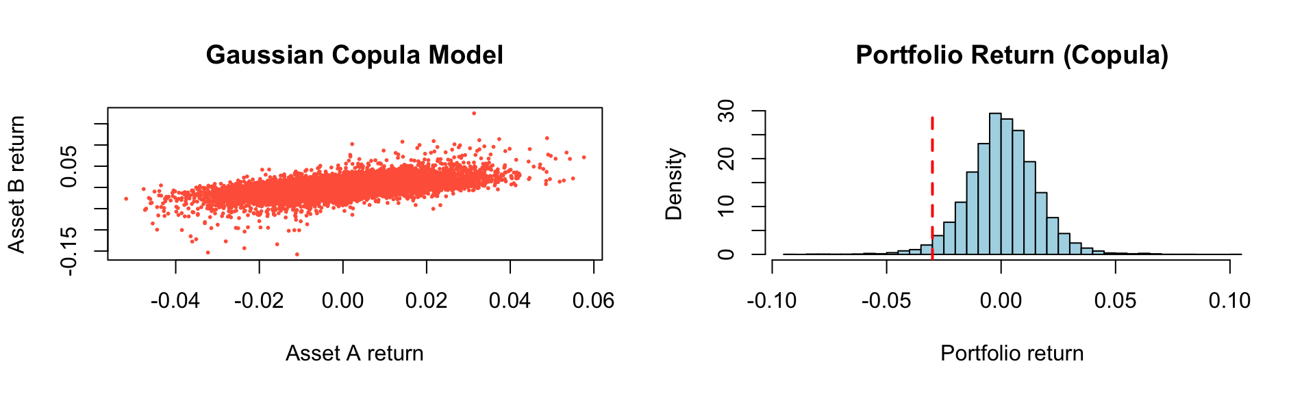
par(mfrow = c(1, 2))

plot(R_copula[,1], R_copula[,2],
     pch = 16, cex = 0.4, col = "tomato",
     main = "Gaussian Copula Model",
     xlab = "Asset A return", ylab = "Asset B return")

hist(port_copula, breaks = 40, freq = FALSE, col = "lightblue",
     main = "Portfolio Return (Copula)",
     xlab = "Portfolio return")
abline(v = -0.03, col = "red", lwd = 2, lty = 2)

Independent Model (Benchmark)

Using the same model setup as Copula-based model, we simulate returns of Asset A and Asset B independently:

set.seed(1234)

R1_ind <- rnorm(n, mean = 0.0005, sd = 0.015)
R2_ind <- 0.0008 + 0.02 * (rt(n, df = 4) / sqrt(2))

R_port_ind <- 0.5 * R1_ind + 0.5 * R2_ind
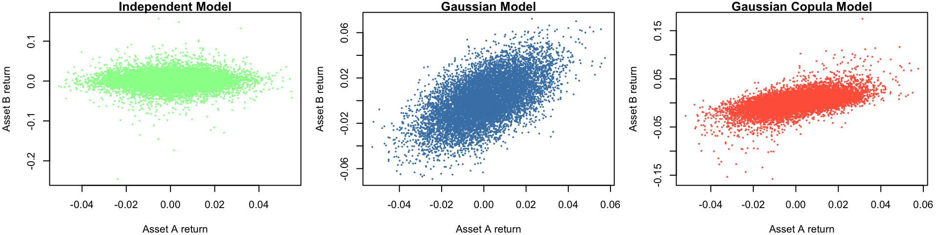
Comparison of Scatterplots
par(mfrow = c(1, 3), mar = c(4,4,1,1))

plot(R1_ind, R2_ind,
     pch = 16, cex = 0.4, col = "palegreen",
     main = "Independent Model",
     xlab = "Asset A return", ylab = "Asset B return")

plot(R_gauss[,1], R_gauss[,2],
     pch = 16, cex = 0.4, col = "steelblue",
     main = "Gaussian Model",
     xlab = "Asset A return", ylab = "Asset B return")

plot(R_copula[,1], R_copula[,2],
     pch = 16, cex = 0.4, col = "tomato",
     main = "Gaussian Copula Model",
     xlab = "Asset A return", ylab = "Asset B return")
  • Independent model → circular cloud → no structure → returns move independently
  • Gaussian model → elliptical cloud → linear dependence
  • Copula model → similar dependence, but more extreme points → heavier tails visible
Comparison of Marginal Histograms
par(mfrow = c(1, 3), mar = c(4,4,1,1))

hist(R_port_ind, breaks = 40, freq = FALSE, col = "lightpink",
     main = "Portfolio Return (Independent)",
     xlab = "Portfolio return")
abline(v = -0.03, col = "red", lwd = 2, lty = 2)

hist(port_gauss, breaks = 40, freq = FALSE, col = "lightgray",
     main = "Portfolio Return (Gaussian)",
     xlab = "Portfolio return")
abline(v = -0.03, col = "red", lwd = 2, lty = 2)

hist(port_copula, breaks = 40, freq = FALSE, col = "lightblue",
     main = "Portfolio Return (Copula)",
     xlab = "Portfolio return")
abline(v = -0.03, col = "red", lwd = 2, lty = 2)
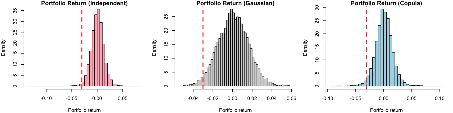
  • Independent → narrow distribution     Gaussian → wider spread     Copula → similar spread, fatter tails


Mean SD VaR_5.5% VaR_1.1% Prob_Loss_gt_3pct
Gaussian 8e-04 0.0155 -0.0248 -0.0352 0.0232
Copula 7e-04 0.0153 -0.0238 -0.0378 0.0235
Independent 6e-04 0.0124 -0.0193 -0.0305 0.0106


  • The means are very similar → expected return is not sensitive to dependence.
  • The standard deviation increases significantly when dependence is introduced.
  • Dependence roughly doubles the probability of large losses.

Value-at-Risk (VaR) is a commonly used measure of downside risk (losses or left tail of the distribution). It measures “How bad can losses be, with a given level of confidence?”

Formally, the VaR at level \(\alpha\) (e.g., 5% or 1%) is the threshold such that:

\[ P(R_p \leq \text{VaR}_\alpha) = \alpha, \]

where \(R_p\) is the portfolio return.

  • VaR (5%) = −0.02 means there is a 5% chance that the portfolio return is worse than −2%.
  • VaR (1%) = −0.04 means there is a 1% chance that the loss exceeds 4%.


Mean SD VaR_5.5% VaR_1.1% Prob_Loss_gt_3pct
Gaussian 8e-04 0.0155 -0.0248 -0.0352 0.0232
Copula 7e-04 0.0153 -0.0238 -0.0378 0.0235
Independent 6e-04 0.0124 -0.0193 -0.0305 0.0106


  • Both dependent models produce more negative VaR than the independent case.
  • The copula model has the worst 1% VaR.

Takeaway: Ignoring dependence underestimates risk. Heavy tails (copula model) increase extreme losses.