Simulation is the systematic use of a computational model to study the behaviour of a system that evolves under uncertainty. More precisely, a simulation replaces analytical derivation or physical experimentation with a carefully constructed algorithm that generates artificial data according to specified probabilistic rules. By observing the behaviour of this artificial system repeatedly, we approximate characteristics of the real system.
The defining feature of simulation is that randomness is built into the mechanism of the model. Unlike deterministic computation, where the same inputs always produce the same outputs, a stochastic simulation produces different outcomes on each run (nondeterministic). This variability is not a flaw but a deliberate feature. It mirrors the variability present in real-world systems and allows us to quantify uncertainty in outcomes.
To understand what simulation achieves, consider the distinction between a single realisation and a distribution of outcomes. Running a queueing system for one simulated day yields one possible history of arrivals and waiting times. Running the simulation thousands of times produces a distribution of possible waiting times. It is this distribution—not any single run—that provides meaningful statistical insight. Simulation therefore shifts our focus from deterministic prediction to probabilistic understanding.
It is important to recognise that a simulation does not replicate reality directly; it replicates a model of reality.
The validity of the conclusions depends entirely on the appropriateness of the modelling assumptions. If the model is unrealistic, the simulation will faithfully reproduce unrealistic behaviour. For this reason, simulation should always be viewed as a structured experiment conducted under explicitly stated assumptions.
A useful way to conceptualise simulation is as a virtual laboratory. In a physical laboratory, we manipulate inputs and observe outputs. In a simulation, we encode the system’s rules into a computer program, manipulate parameters, and observe the resulting behaviour. This makes simulation especially powerful for “what-if” analysis. We can change arrival rates, service mechanisms, volatility parameters, or structural assumptions and immediately study the consequences, often at negligible cost compared to real-world experimentation.
Finally, simulation is inherently approximate. Because we rely on finite repetition, our estimates contain sampling variability. However, probability theory provides the theoretical foundation that guarantees improvement with increased replication. As the number of runs grows, simulated averages stabilise and converge toward their true theoretical values. This convergence justifies the use of simulation as a legitimate inferential tool rather than a heuristic shortcut.
1.2 Simulation Workflow
Problem
→
Model
→
Simulation
→
Analysis
→
Conclusion
Although simulation problems arise in many different domains, the structure of a well-designed simulation study follows a common logical progression. The process begins with problem formulation. The question of interest must be stated clearly and quantitatively. Vague objectives lead to unfocused models and ambiguous conclusions. For example, asking whether “queues are too long” is imprecise; asking for the expected waiting time and the probability that waiting exceeds ten minutes is specific and measurable.
Once the problem is defined, the next step is model construction. This involves identifying the essential components of the system and deciding how to represent them mathematically. In a queueing model, we must specify how customers arrive, how long service takes, how many servers operate, and how customers are prioritised. These assumptions may be based on empirical data, theoretical reasoning, or simplifying approximations. The art of modelling lies in balancing realism with tractability.
After specifying the model, it must be translated into an algorithm. This step converts conceptual assumptions into computational procedures. Random variables must be generated from appropriate distributions, system states must be updated according to explicit rules, and outputs must be recorded systematically. At this stage, verification becomes crucial: we must ensure that the code implements the intended logic correctly.
The simulation is then executed repeatedly. Each run generates one realisation of the system’s behaviour. By aggregating results across many independent replications, we estimate performance measures such as means, variances, quantiles, and probabilities of rare events. Statistical analysis of the output is essential; without it, simulation reduces to uncontrolled numerical experimentation.
Finally, conclusions are drawn and interpreted in the context of the original problem. If results are unsatisfactory or unrealistic, the process returns to earlier stages. Simulation is inherently iterative. Assumptions are revised, parameters are recalibrated, and models are refined. This feedback loop is not a sign of failure but a central feature of responsible modelling.
1.3 Simulation vs Analytical Solutions
Simulation and analytical methods represent two fundamentally different approaches to solving quantitative problems.
Analytical solutions rely on mathematical derivations that express relationships in closed form.
When available, such solutions provide exact expressions that reveal structural properties of the system. They are often elegant, computationally efficient, and theoretically satisfying.
However, analytical solutions typically require strong assumptions. Many real-world systems violate the simplifying conditions necessary for closed-form derivations. Introducing heterogeneous agents, time-varying dynamics, nonlinear interactions, or complex dependence structures often renders analytical treatment infeasible.
Simulation, by contrast, replaces algebraic derivation with computational experimentation.
Rather than solving equations, we approximate quantities of interest by averaging outcomes from repeated random experiments. The result is approximate rather than exact, but the method accommodates far greater structural complexity. Simulation therefore trades exactness for flexibility.
The choice between analytical and simulation approaches is not a matter of superiority but of suitability. When exact formulas exist and assumptions are reasonable, analytical solutions are often preferable. When systems are too complex for tractable mathematics, simulation becomes indispensable. In practice, the two approaches complement one another: analytical results guide modelling intuition, while simulation explores behaviour beyond analytical reach.
Analytical Solutions
Simulation
Nature
Nature
Formulas/exact, showing how variables relate
Produces approximate answers
Strong assumptions
Handles complex, realistic systems
Often elegant and fast to compute
Requires computational power
Flexible: you can model almost anything
When to Use
When to Use
The system is simple enough to model with equations
The system is too complicated for closed-form math
The mathematics is tractable
You want to include realistic randomness
You need exact results
You want to test “what-if” scenarios
You want to understand the structure of the problem
You need distributions, not just averages
Example
Example
For a simple queue with arrival rate \(\lambda\) and service rate \(\mu\), the average number of customers in the system is: \[L = \frac{\lambda}{\mu - \lambda}\]
If the café has: • two baristas with different speeds • customers who sometimes abandon the queue
1.4 Random Number Generation
All stochastic simulation depends on our ability to generate random numbers. Without randomness, simulation reduces to deterministic computation and cannot represent uncertainty. Yet computers are deterministic machines: given the same inputs, they always produce the same outputs. This raises an important question: how can a deterministic machine generate randomness?
The answer lies in the concept of pseudorandomness. Computers do not generate truly random numbers in the physical sense. Instead, they generate sequences of numbers using deterministic algorithms designed to mimic the statistical properties of randomness. These algorithms are known as pseudorandom number generators (PRNGs).
A PRNG begins with an initial value called a seed. It then applies a recursive formula to produce a sequence of numbers that appear random. If the same seed is used, the same sequence will be generated. This reproducibility is not a weakness; it is one of the greatest strengths of computational simulation. It allows experiments to be replicated exactly, facilitating debugging, validation, and scientific transparency.
True randomness, by contrast, arises from inherently unpredictable physical processes such as radioactive decay, atmospheric noise, or quantum phenomena. Such randomness is nondeterministic. While it is possible to use hardware devices to capture physical randomness, simulation typically relies on algorithmic generators because they are fast, reproducible, and sufficiently random for statistical purposes.
For a pseudorandom sequence to be useful in simulation, it must satisfy several important properties. The sequence should have a very long period before repeating. Its values should be uniformly distributed over the intended range. There should be no detectable patterns or correlations that could bias simulation results. Poor-quality generators can produce subtle dependencies that distort high-dimensional simulations, particularly in Monte Carlo integration or Bayesian computation.
Modern statistical software such as R and Python uses high-quality PRNGs by default. Nevertheless, understanding their structure is essential because every simulated random variable ultimately depends on these underlying generators.
1.4.1 Linear Congruential Generators (LCGs)
One of the earliest and simplest pseudorandom number generators is the Linear Congruential Generator (LCG). Historically important in the development of Monte Carlo methods, the LCG illustrates the basic mechanism of algorithmic randomness.
An LCG generates a sequence of integers according to the recurrence relation:
\[X_{n+1} = (aX_n + c) \ \text{mod} \ m,\]
where \(X\) is the sequence of pseudo-random numbers, \(m\) is the modulus, \(a\) is the multiplier, \(c\) is the increment, and \(X_0\) is the seed. Also,
the modulus \(m, 0 < m\)
the multiplier \(a, 0 < a < m\)
the increment \(c, 0 \leq c < m\)
the seed or start values \(X_0, 0 \leq X_0 < m\)
The modulo operation ensures that the sequence remains within the range \(0 \leq X_n < m\).
Modulo arithmetic
In arithmetic, the modulus refers to the operation that returns the remainder after division.
\[a \bmod m = \text{remainder when } a \text{ is divided by } m\]
Examples:
\(7 \bmod 5 = 2\)
\(5 \bmod 5 = 0\)
\(17 \bmod 5 = 2\)
To use the sequence for simulation, the generated integers are typically scaled to the interval (0,1) by dividing by \(m\). This produces numbers that approximate draws from a Uniform(0,1) distribution.
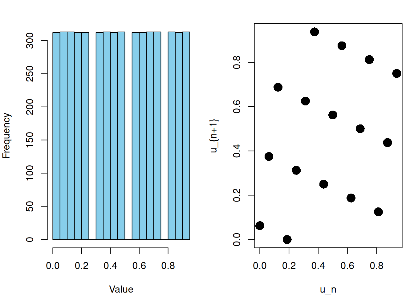
Although the formula is simple, the choice of parameters \(a\), \(c\), and \(m\) critically determines the quality of the generator. Poor parameter choices can produce short cycles and visible lattice structures when successive pairs \((X_n, X_{n+1})\) are plotted. These patterns indicate correlation and undermine the reliability of simulations.
Example: Bad LCG with poor parameter choices
lcg <-function(n, seed =1, a =5, c =1, m =16) { x <-numeric(n) x[1] <- seedfor (i in2:n) { x[i] <- (a * x[i-1] + c) %% m } u <- x / m # convert to Uniform(0,1)return(u)}set.seed(123)u <-lcg(5000)par(mfrow=c(1,2), mar =c(4, 4, 2, 1))hist(u, breaks =30, col ="skyblue",xlab ="Value", main ="")plot(u[-length(u)], u[-1], pch =16, cex =2, xlab ="u_n", ylab ="u_{n+1}")
While LCGs are computationally efficient and easy to implement, they suffer from structural weaknesses. In high-dimensional simulations, they may exhibit undesirable correlations. For this reason, LCGs are primarily of pedagogical and historical interest rather than practical use in modern statistical computing.
1.4.2 Uniform(0,1) Random Number (Mersenne Twister)
Modern simulation relies on far more sophisticated generators. The most widely used PRNG in contemporary statistical software is the Mersenne Twister, which serves as the default generator in R, Python (NumPy), MATLAB, and many other systems.
The Mersenne Twister was designed to have an extremely long period (specifically \(2^{19937} - 1\)), excellent equidistribution properties, and strong performance in high-dimensional settings. For most practical simulation tasks, it provides randomness of sufficient quality.
set.seed(123)u <-runif(1000, 0, 1)par(mfrow=c(1,2), mar =c(4, 4, 2, 1))plot(u, pch =16, col ="darkgreen", cex=.8,main ="Uniform(0,1) Random Draws",xlab ="Index", ylab ="Value")hist(u,breaks =20,col ="skyblue",main ="Histogram of Uniform(0,1) Samples",xlab ="Value",ylab ="Frequency",freq =FALSE,)lines(density(u), col ="blue", lwd =2)
The fundamental output of nearly all PRNGs is a sequence of values that approximate independent draws from the Uniform(0,1) distribution. This distribution plays a central role in simulation because it serves as the building block for generating all other random variables.
If we can generate \(U \sim \text{Uniform}(0,1)\), we can transform it to simulate other distributions. For example,
A Bernoulli(\(p\)): returning 1 if \(U < p\) and 0 otherwise.
An Exponential(\(\lambda\)): using the inverse transform \(X = -\frac{1}{\lambda} \ln(1 - U)\).
A Normal(0, 1): using transformations such as the Box–Muller method.
This principle — generating complex distributions from uniform random numbers — underlies nearly all simulation techniques studied in this unit. Whether we simulate queueing systems, perform Monte Carlo (MC) integration, or implement Markov Chain Monte Carlo (MCMC) algorithms, the process always begins with high-quality Uniform(0,1) draws.
In this sense, the uniform random number generator is the engine of stochastic simulation. If that engine is flawed, every subsequent simulation result is compromised. If it is reliable, we can build complex probabilistic models with confidence.
 Scatter-1.png)