36  Autocorrelation Function

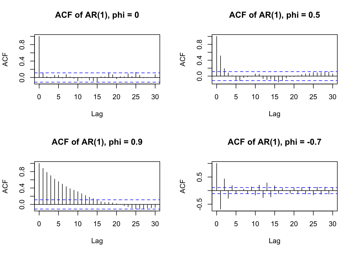
So far, we have described temporal dependence visually and intuitively: some processes show persistence, some oscillate, and some behave almost like white noise. To measure this dependence more systematically, we use the autocorrelation function, or ACF.

The ACF is a general tool used to measure temporal dependence in any time series. We first study it in the context of AR(1), where it has a particularly simple form.

The ACF measures the correlation between a time series and a lagged version of itself.

For a time series \(X_t\), the lag-\(k\) autocorrelation is

\[ \rho_k = \text{Corr}(X_t, X_{t-k}). \]

Here, \(k\) is called the lag.

For example:

• lag 1 measures dependence between \(X_t\) and \(X_{t-1}\),
• lag 2 measures dependence between \(X_t\) and \(X_{t-2}\),
• lag 3 measures dependence between \(X_t\) and \(X_{t-3}\).

The ACF tells us how strongly the past is connected to the present.

• If autocorrelations are close to zero, the process has little memory.
• If autocorrelations decay slowly, shocks persist for a long time.
• If autocorrelations alternate between positive and negative values, the process oscillates.

For white noise,

\[ \rho_k = 0 \quad \text{for all } k > 0, \]

because observations at different times are independent.

For a stationary AR(1) process,

\[ X_t = \phi X_{t-1} + \varepsilon_t, \]

the theoretical ACF is

\[ \rho_k = \phi^k. \]

This is the same geometric decay pattern we observed in shock propagation.

The value of \(\phi\) also determines the shape of the ACF:

Value of \(\phi\)	ACF behaviour	Interpretation
\(\phi = 0\)	zero after lag 0	white noise
\(0 < \phi < 1\)	positive decay	persistence
\(\phi \approx 1\)	slow decay	long memory
\(\phi < 0\)	alternating signs	oscillation

Thus, the ACF provides a numerical and visual way to diagnose temporal dependence.

Example: Compare the ACF of AR(1) processes with different values of \(\phi\).

set.seed(1234)

n <- 300
phis <- c(0, 0.5, 0.9, -0.7)

simulate_ar1 <- function(phi, n) {
  epsilon <- rnorm(n, mean = 0, sd = 1)
  X <- numeric(n)
  X[1] <- 0
  
  for (t in 2:n) {
    X[t] <- phi * X[t - 1] + epsilon[t]
  }
  
  return(X)
}

par(mfrow = c(2, 2))

for (phi in phis) {
  X <- simulate_ar1(phi, n)
  acf(
    X,
    main = paste("ACF of AR(1), phi =", phi),
    lag.max = 30
  )
}

import numpy as np
import matplotlib.pyplot as plt
from statsmodels.graphics.tsaplots import plot_acf

np.random.seed(1234)

n = 300
phis = [0, 0.5, 0.9, -0.7]

def simulate_ar1(phi, n):
    epsilon = np.random.normal(0, 1, n)
    X = np.zeros(n)
    
    for t in range(1, n):
        X[t] = phi * X[t - 1] + epsilon[t]
    
    return X

fig, axes = plt.subplots(2, 2, figsize=(10, 6))

for ax, phi in zip(axes.flatten(), phis):
    X = simulate_ar1(phi, n)
    plot_acf(X, lags=30, ax=ax)
    ax.set_title(f"ACF of AR(1), phi = {phi}")

plt.tight_layout()
plt.show()

• When \(\phi = 0\), the process is white noise. The autocorrelations are close to zero for all non-zero lags.

• When \(\phi = 0.5\), the ACF decays fairly quickly. This indicates moderate short-term memory.

• When \(\phi = 0.9\), the ACF decays slowly. This indicates strong persistence: values far apart in time are still related.

• When \(\phi = -0.7\), the ACF alternates between positive and negative values. This reflects oscillating behaviour in the time series.

The ACF connects the visual behaviour of a time series to a diagnostic tool:

Persistence appears as slowly decaying autocorrelation, while oscillation appears as alternating positive and negative autocorrelation.

This makes the ACF a natural bridge between simulation, interpretation, and diagnosis.