Simulation is built upon the ability to generate random variables with specified probability distributions. Before developing simulation algorithms, we must revisit the mathematical structure of univariate distributions and clarify the probabilistic ideas that underlie them.
A random variable is a numerical function defined on a sample space,
\[X : \Omega \to \mathbb{R},\]
which assigns a real number to each outcome of a random experiment. In simulation, random variables are the primary objects we generate. Their distributions determine the behaviour of the systems we model.
Random variables may be discrete or continuous, and while the computational treatment differs slightly between these two cases, the underlying principles are unified.
6.1 Discrete Distributions
Discrete distributions arise naturally whenever we simulate events, counts, or categorical outcomes. Each of the following plays a distinct structural role in modelling stochastic systems.
We can categorise discrete distributions into four groups:
The cumulative distribution function (CDF) is defined by
\[F(x) = P(X \le x) = \sum_{t \le x} p(t).\]
The CDF plays a central role in simulation theory, as it links probability with transformation methods that we will study later.
6.1.1 Bernoulli Distribution
The simplest discrete distribution is the Bernoulli distribution. A Bernoulli random variable represents a single trial with two possible outcomes, often labelled 1 (success) and 0 (failure).
Why it matters in simulation:
It is the atomic unit of discrete randomness.
Many complex models are constructed from repeated Bernoulli trials.
It can be used to represent a (possibly biased) coin toss where 1 and 0 would represent “heads” and “tails”, respectively, and \(p\) would be the probability of the coin landing on heads (or vice versa).
If \(X\) is an independent Bernoulli experiment with a probability of success \(p\): \[X \sim \text{Bernoulli}(p)\]
then the PMF of this distribution, over possible outcomes \(k\), is \[
P(X=x) = p^x(1-p)^{1-x} \quad \text{for } x \in \{0,1\}.
\]\[P(X=1)=p, \quad P(X=0)=q=1-p.\]
The CDF of the distribution is given by \[
F(x) = \begin{cases}
0 & x<0, \\
1-p & 0 \leq x \lt 1, \\
1 & x \geq 1.
\end{cases}
\]
Its expectation and variance are \[\mathbb{E}[X]=p, \qquad \mathrm{Var}(X)=p(1-p)=pq.\]
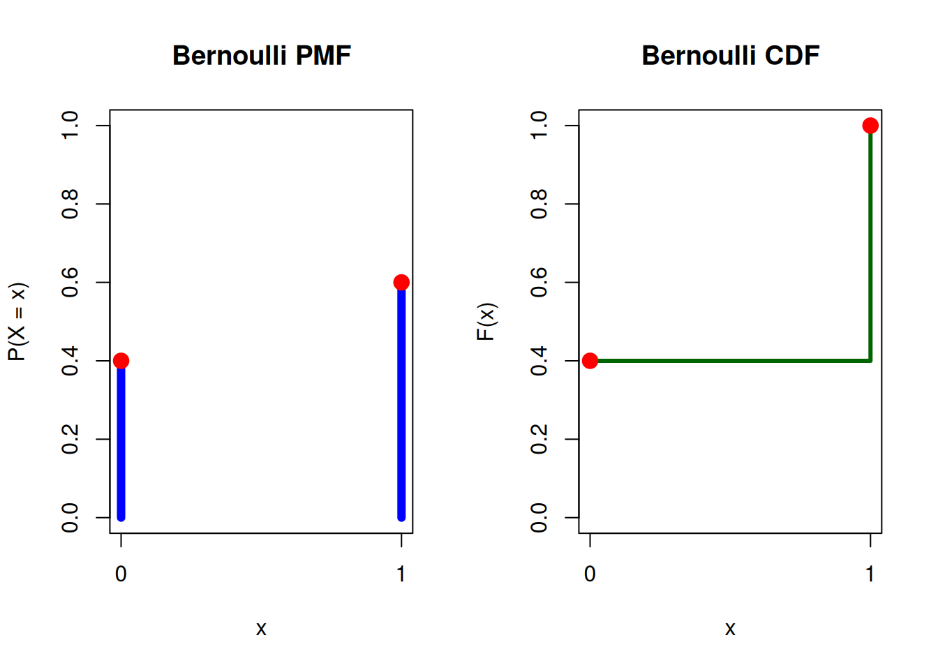
Example: The following plots show the PMF and CDF of a biased coin with a 60% probability of landing heads (success).
Bernoulli(0.6) PMF and CDF
# Parameterp <-0.6# Probability of success# Possible valuesx <-c(0, 1)# PMF and CDFpmf <-dbinom(x, size =1, prob = p)cdf <-pbinom(x, size =1, prob = p)# Set plotting area to 1 row, 2 columnspar(mfrow =c(1, 2))# --- PMF Plot ---plot(x, pmf,type ="h",lwd =6,col ="blue",ylim =c(0, 1),xaxt ="n",main ="Bernoulli PMF",xlab ="x",ylab ="P(X = x)")axis(1, at = x) # manually adds tick markspoints(x, pmf, pch =19, col ="red", cex =1.5)# --- CDF Plot ---plot(x, cdf,type ="s",lwd =3,col ="darkgreen",ylim =c(0, 1),xaxt ="n",main ="Bernoulli CDF",xlab ="x",ylab ="F(x)")axis(1, at = x) # manually adds tick markspoints(x, cdf, pch =19, col ="red", cex =1.5)
Advanced: Using Plotly to create an interactive plot for different values of \(p\), where \(0 \leq p \leq 1\):
Bernoulli(p) with an interactive p slider
library(plotly)library(dplyr)library(tidyr)# Grid of p values for the sliderp_vals <-seq(0, 1, by =0.1)x_vals <-c(0, 1)# Precompute PMF and CDF for all p (browser-only interactivity; no recomputation)df <-expand_grid(p = p_vals, x = x_vals) %>%mutate(pmf =dbinom(x, size =1, prob = p),cdf =pbinom(x, size =1, prob = p),frame =sprintf("p = %.2f", p),x_chr =as.character(x) # helps bar chart labeling )# --- PMF (bar-like) ---pmf_fig <- df %>%plot_ly(x =~x_chr, y =~pmf,frame =~frame,type ="bar",marker =list(color ="steelblue"),hovertemplate ="x=%{x}<br>P(X=x)=%{y:.2f}<extra></extra>" ) %>%layout(title =list(text ="Bernoulli PMF"),xaxis =list(title ="x", categoryorder ="array", categoryarray =c("0","1")),yaxis =list(title ="P(X = x)", range =c(0, 1)) )# --- CDF (step + points) ---cdf_fig <- df %>%plot_ly(x =~x, y =~cdf,frame =~frame,type ="scatter",mode ="lines+markers",line =list(color ="darkgreen", width =3, shape ="hv"),marker =list(color ="red", size =8),hovertemplate ="x=%{x}<br>F(x)=%{y:.2f}<extra></extra>" ) %>%layout(title =list(text ="Bernoulli CDF"),xaxis =list(title ="x", tickmode ="array", tickvals =c(0,1)),yaxis =list(title ="F(x)", range =c(0, 1)) )# Combine side-by-side and add slider + play/pausefig <-subplot(pmf_fig, cdf_fig, nrows =1, shareX =FALSE, titleX =TRUE, titleY =TRUE) %>%layout(title =list(text ="Bernoulli Distribution (interactive p slider)"),showlegend =FALSE ) %>%animation_opts(frame =0, transition =0, redraw =TRUE) %>%animation_slider(currentvalue =list(prefix ="")) %>%animation_button(x =1, xanchor ="right", y =0, yanchor ="bottom")fig
6.1.2 Binomial Distribution
The Binomial distribution counts the number of successes in \(n\) independent Bernoulli trials.
Why it matters in simulation:
Models aggregated binary outcomes.
Appears in reliability systems (number of working components).
Used in bootstrap and resampling procedures.
Forms a bridge between Bernoulli and Poisson processes.
In simulation studies, binomial counts often measure performance metrics across repeated trials.
If we repeat a Bernoulli experiment with probability of success equal to \(p\) for \(n\) times independently, the number of successes\(X\) follows a Binomial distribution: \[X \sim \text{Binomial}(n,p),\] with PMF and CDF\[P(X=k)=\binom{n}{k}p^k(1-p)^{n-k}, \qquad
\sum_{k=0}^x P(X=k).
\]
The expectation and variance are \[\mathbb{E}[X]=np, \qquad \mathrm{Var}(X)=np(1-p).\]
In simulation, the Binomial distribution often models counts of events within fixed trials. For example, defect counts in manufacturing or successful transmissions in a network.
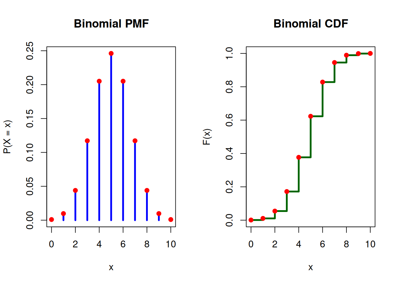
Example: Suppose you flip a fair coin 10 times. Each flip has a 50% chance of landing heads, and the flips are independent. Let X be the number of heads obtained in the 10 flips. The PMF plot shows the probability of obtaining each possible number of successes. Each point on the CDF plot gives the cumulative probability up to that value.
Binomial(10, 0.5) PMF and CDF
# Parametersn <-10# number of trialsp <-0.5# probability of success# Possible valuesx <-0:n# PMF and CDFpmf <-dbinom(x, size = n, prob = p)cdf <-pbinom(x, size = n, prob = p)# Set plotting area: 1 row, 2 columnspar(mfrow =c(1, 2))# --- PMF Plot ---plot(x, pmf,type ="h",lwd =3,col ="blue",main ="Binomial PMF",xlab ="x",ylab ="P(X = x)",ylim =c(0, max(pmf)))points(x, pmf, pch =19, col ="red")# --- CDF Plot ---plot(x, cdf,type ="s",lwd =3,col ="darkgreen",main ="Binomial CDF",xlab ="x",ylab ="F(x)",ylim =c(0, 1))points(x, cdf, pch =19, col ="red")
Advanced: Using Plotly to create an interactive plot for different values of \(p\), where \(0 \leq p \leq 1\):
Binomial(10,p) with an interactive p slider
library(plotly)library(dplyr)library(tidyr)n <-10p_vals <-seq(0, 1, by =0.1) # coarser slider; change to 0.01 if you want smootherx_vals <-0:ndf <-expand_grid(p = p_vals, x = x_vals) %>%mutate(pmf =dbinom(x, size = n, prob = p),cdf =pbinom(x, size = n, prob = p),frame =sprintf("p = %.2f", p) )pmf_fig <- df %>%plot_ly(x =~x, y =~pmf,frame =~frame,type ="bar",marker =list(color ="steelblue"),hovertemplate ="x=%{x}<br>P(X=x)=%{y:.4f}<extra></extra>" ) %>%layout(title =list(text =paste0("Binomial PMF (n = ", n, ")")),xaxis =list(title ="x", dtick =2),yaxis =list(title ="P(X = x)") )cdf_fig <- df %>%plot_ly(x =~x, y =~cdf,frame =~frame,type ="scatter",mode ="lines+markers",line =list(color ="darkgreen", width =3, shape ="hv"),marker =list(color ="red", size =7),hovertemplate ="x=%{x}<br>F(x)=%{y:.4f}<extra></extra>" ) %>%layout(title =list(text =paste0("Binomial CDF (n = ", n, ")")),xaxis =list(title ="x", tickmode ="array", tickvals =seq(0, n, by =2)),yaxis =list(title ="F(x)", range =c(0, 1)) )fig <-subplot(pmf_fig, cdf_fig, nrows =1, shareX =FALSE, titleX =TRUE, titleY =FALSE) %>%layout(title =list(text ="Binomial Distribution (interactive p slider)"),showlegend =FALSE,margin =list(l =90, r =30, t =70, b =55),yaxis =list(title ="P(X = x)", title_standoff =15),yaxis2 =list(title ="F(x)", title_standoff =15) ) %>%animation_opts(frame =0, transition =0, redraw =TRUE) %>%animation_slider(currentvalue =list(prefix ="")) %>%animation_button(x =1, xanchor ="right", y =0, yanchor ="bottom")fig
6.1.3 Geometric Distribution
The Geometric distribution models the number of trials required until the first success. in a sequence of independent Bernoulli trials, where each trial has a constant probability of success.
Why it matters in simulation:
Represents waiting times in discrete-time systems.
Discrete analogue of the exponential distribution.
Possesses the memoryless property, making it important in stochastic process theory.
Useful in modelling repeated attempts (e.g., retry mechanisms in networks).
If \(X\) is the number of trials (independent and identical Bernoulli experiment) required to get first success, and \(p\) is the success probability (\(0 < p \leq 1\)), then \[X \sim \text{Geo}(p)\]
The PMF of a geometric distribution (the probability that the \(k\)-th trial is the first success) is given by:
\[P(X = k) = (1 - p)^{k - 1} p\]
for \(k\in \mathbb{N}={1,2,3,...}\).
The CDF of a geometric distribution is given by:
\[P(X \leq k) = 1 - (1 - p)^k\]
The mean and variance of a geometric distribution are:
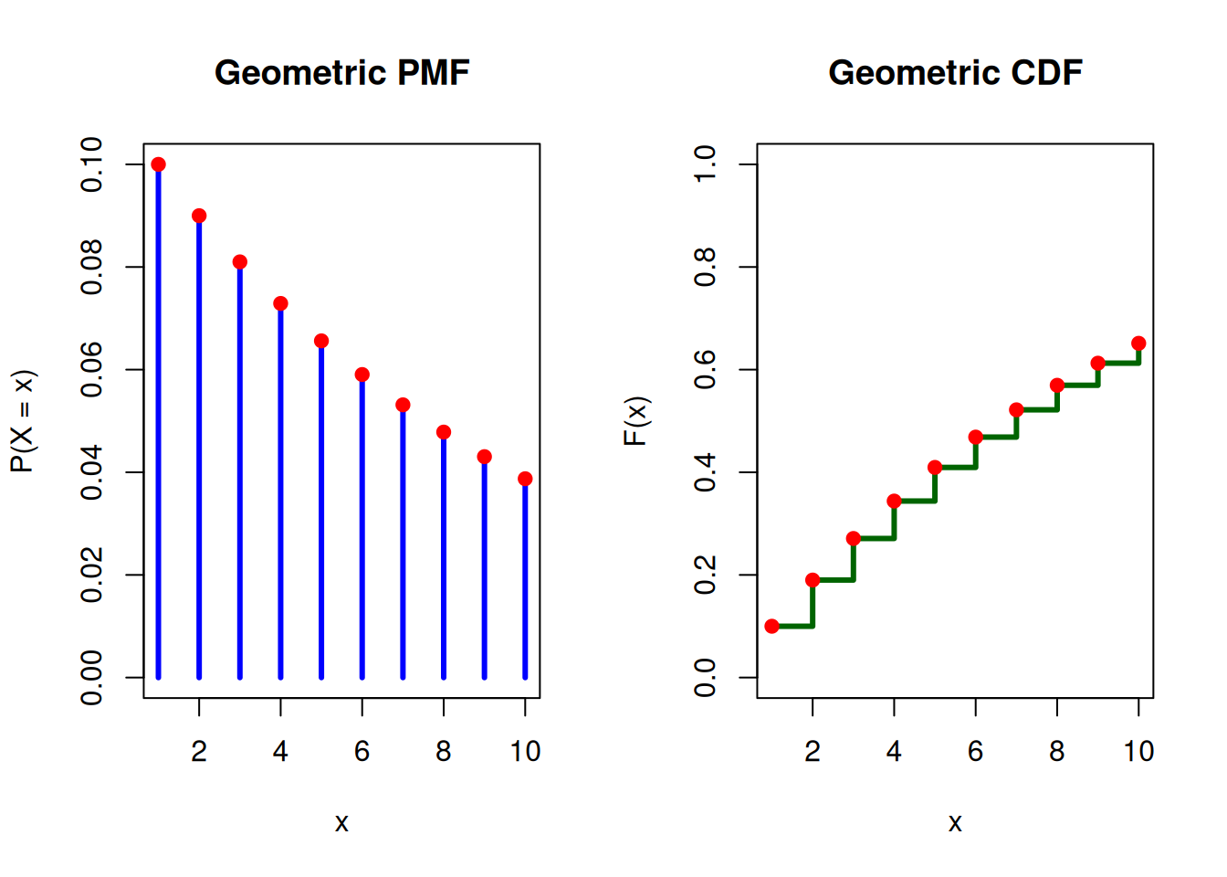
Example: An oil company conducts a geological study that indicates exploratory oil wells in a region have 10% chance of striking oil. The PMF plot shows the probability that the first strike will come on an \(X-1\) well, and the CDF plot gives the cumulative probability up to that value.
Warning: Built-in geometric distribution functions in R model the number of failures before success occurs; therefore, we model \(X-1\) for \(k \in \mathbb{N_0} = \{0,1,2,...\}.\)
What is the probability that first strike comes on a third well?
dgeom(x =2, prob =0.1)
[1] 0.081
Geometric(0.1) PMF and CDF
# Parametersn <-10# number of trialsp <-0.1# probability of success# Possible valuesx <-1:n# PMF and CDFpmf <-dgeom(x-1, prob = p)cdf <-pgeom(x-1, prob = p)# Set plotting area: 1 row, 2 columnspar(mfrow =c(1, 2))# --- PMF Plot ---plot(x, pmf,type ="h",lwd =3,col ="blue",main ="Geometric PMF",xlab ="x",ylab ="P(X = x)",ylim =c(0, max(pmf)))points(x, pmf, pch =19, col ="red")# --- CDF Plot ---plot(x, cdf,type ="s",lwd =3,col ="darkgreen",main ="Geometric CDF",xlab ="x",ylab ="F(x)",ylim =c(0, 1))points(x, cdf, pch =19, col ="red")
Note: The plots above are generated using x = x-1 to model the number of trialsl.
6.1.4 Negative Binomial Distribution
The Negative Binomial generalises the geometric distribution to the number of trials before \(r\) successes.
Why it matters in simulation:
Models overdispersed count data (variance greater than mean).
Frequently used in arrival modelling when Poisson assumptions are too restrictive.
Arises as a mixture of Poisson distributions (important in Bayesian modelling).
In simulation, it allows realistic modelling of variability beyond simple Poisson assumptions.
Let \(X\) be the number of trials (independent and identical Bernoulli experiments) required to achieve \(r\) successes in independent Bernoulli trials with success probability \(p\), then
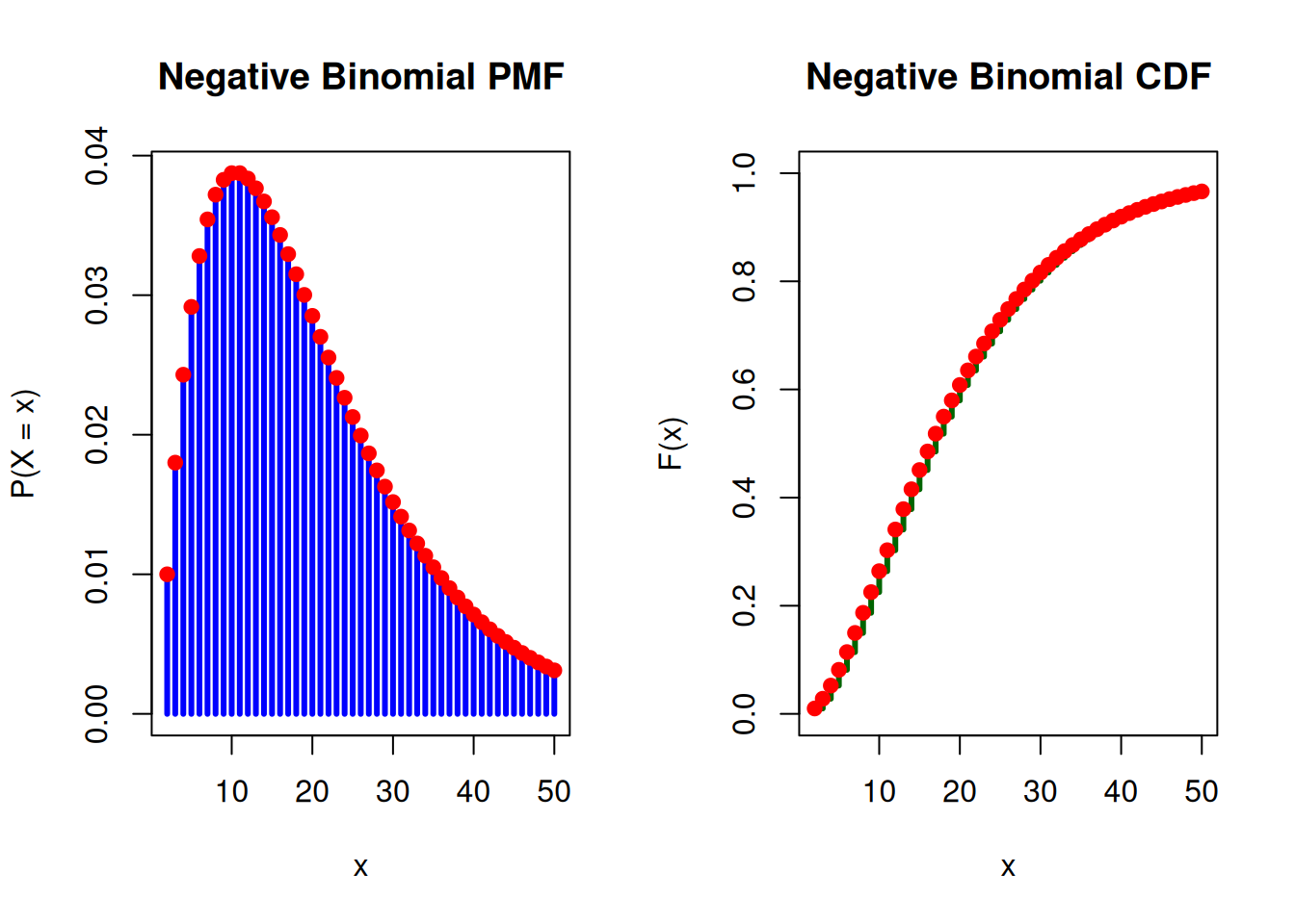
Example: We can use the same example as seen in the Geometric Distribution section. Previously, an oil company conducts a geological study that indicates exploratory oil wells in a region have 10% chance of striking oil. Now we can model the PMF, the probability that \(r\)-th strike comes on \(X\)-th well, and the corresponding CDF.
Warning: Same as geometric distribution, negative binomial distribution functions in R model the number of failures before success occurs; therefore, we model \(X-r\) for \(r > 0.\)
What is the probability that second strike comes on seventh well?
dnbinom(x =7-2, size =2, prob =0.1)
[1] 0.0354294
NegBin(2,0.1) PMF and CDF
# Parametersmax_x <-50# number of trialsr <-2# number of successesp <-0.1# probability of success# Possible valuesx <- r:max_x# PMF and CDFpmf <-dnbinom(x-r, size = r, prob = p)cdf <-pnbinom(x-r, size = r, prob = p)# Set plotting area: 1 row, 2 columnspar(mfrow =c(1, 2))# --- PMF Plot ---plot(x, pmf,type ="h",lwd =3,col ="blue",main ="Negative Binomial PMF",xlab ="x",ylab ="P(X = x)",ylim =c(0, max(pmf)))points(x, pmf, pch =19, col ="red")# --- CDF Plot ---plot(x, cdf,type ="s",lwd =3,col ="darkgreen",main ="Negative Binomial CDF",xlab ="x",ylab ="F(x)",ylim =c(0, 1))points(x, cdf, pch =19, col ="red")
6.1.5 Poisson Distribution
The Poisson distribution arises naturally in modelling the number of events occurring, \(X\), in a fixed interval of time or space.
Why it matters in simulation:
Fundamental to queueing theory.
Governs random arrival systems.
Provides a natural approximation to binomial counts with rare events.
Plays a central role in discrete-event simulation.
Many simulation models begin with:
“Assume arrivals follow a Poisson process.”
If events occur independently at a constant average rate \(\lambda\), then
A distinctive feature is that both expectation and variance,
\[\mathbb{E}[X]=\mathrm{Var}(X)=\lambda.\]
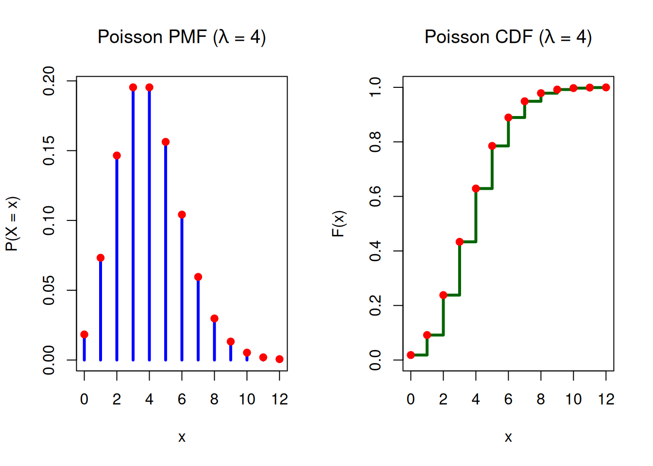
Example: Suppose customers arrive at a service desk at an average rate of 4 customers per hour. Assume arrivals occur independently and at a constant average rate. The PMF plot shows the probability of observing each possible number of arrivals in one hour. Each point on the CDF plot gives the cumulative probability of observing at most that many arrivals.
\[\mathbb{E}[X_i] = n p_i, \quad \mathrm{Var}(X_i) = n p_i (1 - p_i).\]
This resembles the binomial mean and variance because each \(X_i\) marginally follows \(X_i \sim \text{Binomial}(n,p_i)\)
Example: Suppose we roll a fair six-sided die \(n = 10\) times. Each roll results in one of 6 possible outcomes. Each outcome has probability of 1/6. Let \(X_i\) be number of times face \(i\) appears in 10 rolls. Then,
What is the probability that the 10 rolls result in:
1 appears 2 times
2 appears 1 time
3 appears 3 times
4 appears 0 times
5 appears 2 times
6 appears 2 times
So, \((x_1,x_2,x_3,x_4,x_5,x_6) = (2,1,3,0,2,2)\)
The probability of this exact configuration is
\[
P =
\frac{10!}{2!1!3!0!2!2!}
\left(\frac16\right)^{10}.
\]
dmultinom(x =c(2,1,3,0,2,2), prob =rep(1/6, 6))
[1] 0.001250286
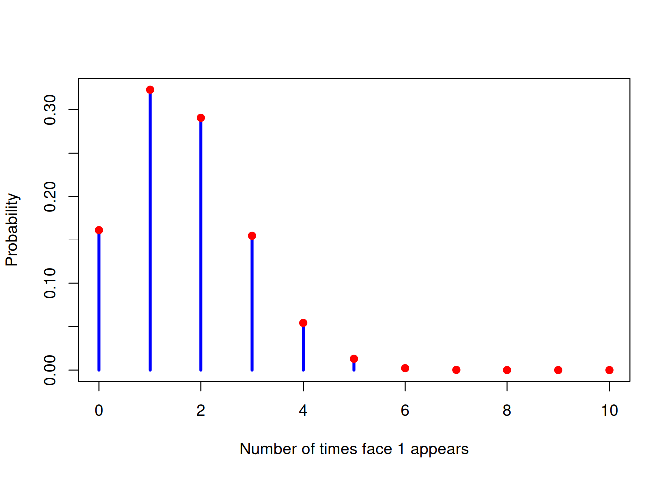
The multinomial distribution is multivariate, so it does not have a simple 1D PMF curve like the binomial or Poisson. We must decide what we want to visualise. If we visualise a marginal distribution of one face \(X_i \sim \text{Binomial}(10,1/6)\), it will look just like the same old binomial distribution.
Marginal Distribution of \(X_1\)
n <-10p <-1/6k <-0:npmf <-dbinom(k, size = n, prob = p)plot(k, pmf,type ="h",lwd =3,col ="blue",xlab ="Number of times face 1 appears",ylab ="Probability",ylim =c(0, max(pmf)))points(k, pmf, pch =19, col ="red")
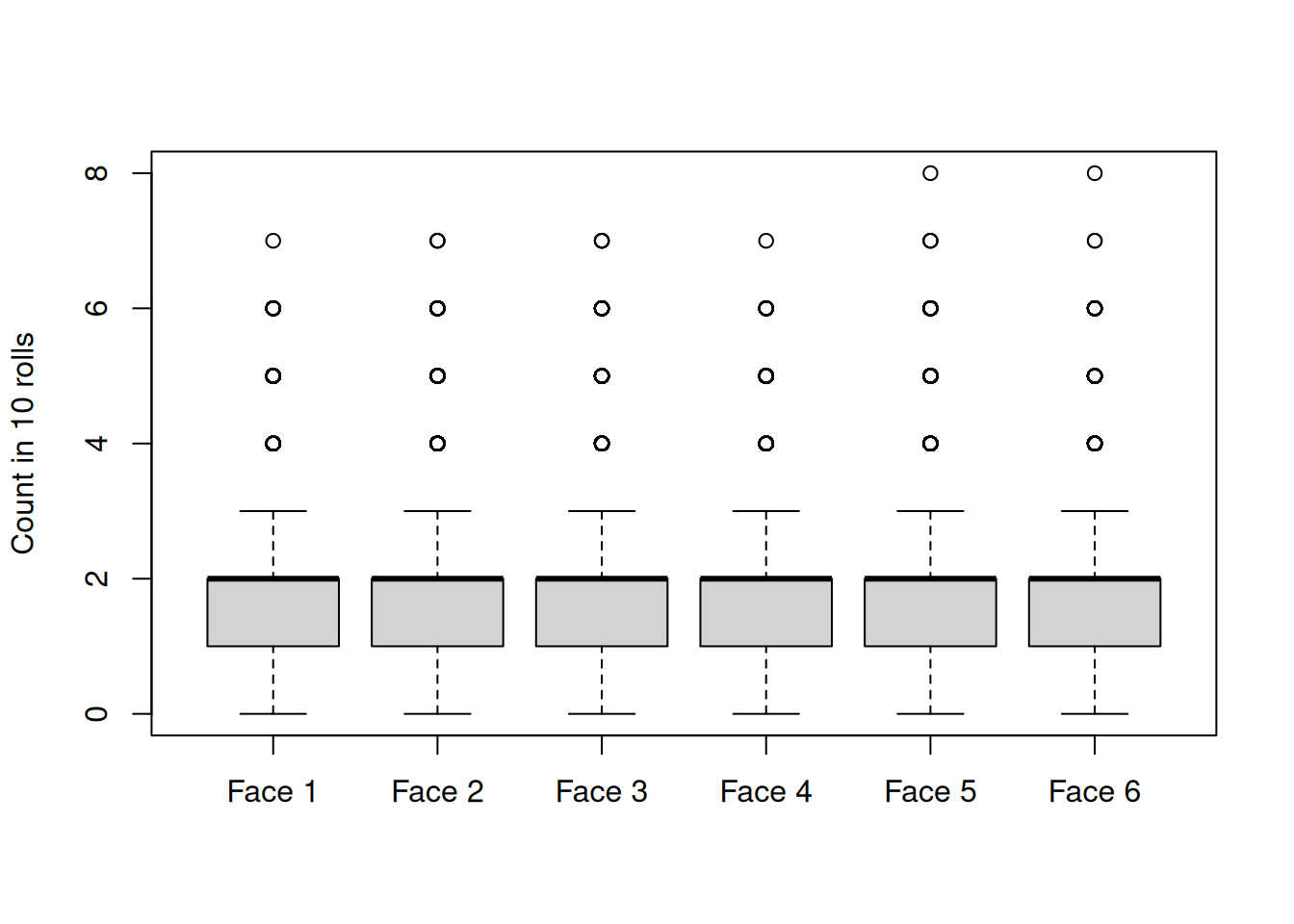
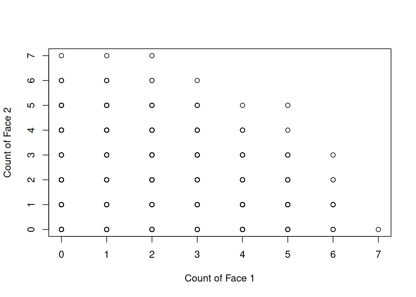
Instead, we can try simulating many multinomial experiments and visualise the counts.
Complex distributions are often constructed from simpler ones.
Unlike discrete variables, continuous random variables assign probability to intervals rather than individual points. Their distribution is described by a probability density function (PDF), \(f(x)\), satisfying
The CDF is always non-decreasing and continuous from the right. Importantly, it provides the bridge between probability theory and simulation algorithms.
6.2.1 Uniform Distribution
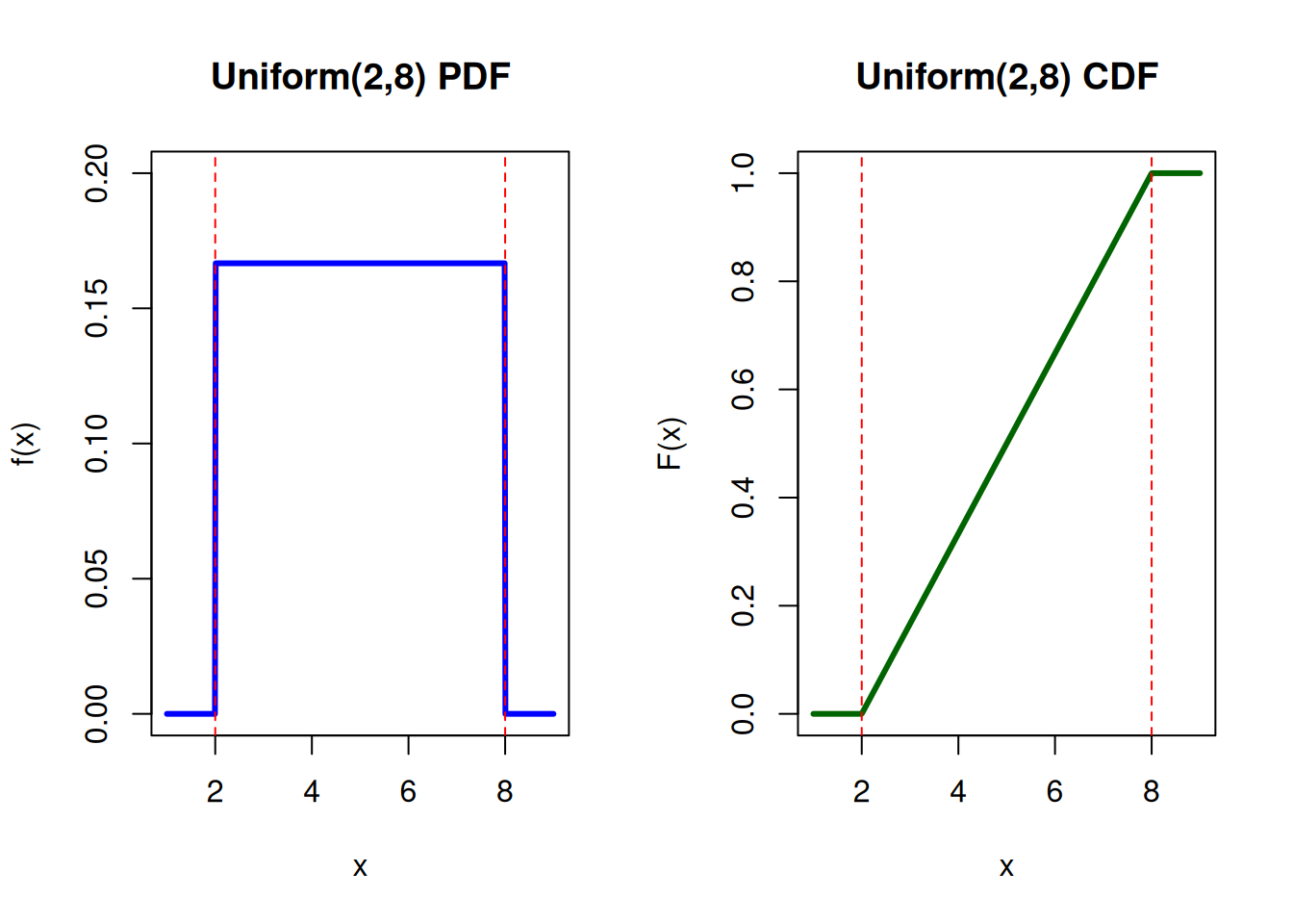
Uniform is a distribution where all outcomes in the range \([a,b]\) are equally likely.
Why it matters in simulation:
All inverse transform methods start from Uniform(0,1).
Acceptance–rejection relies on uniform draws.
Monte Carlo integration uses uniform sampling.
Random number generators are designed to approximate Uniform(0,1).
In simulation theory, Uniform(0,1) is the “raw material” from which all randomness is manufactured.
For \[
X \sim \text{Uniform}(a,b),
\]
the PDF is defined by
\[
f(x)=
\begin{cases}
\dfrac{1}{b-a} & a\leq x \leq b \\
0 & x < a \;\text{ or }\; x > b,
\end{cases}
\]
and the CDF is given by
\[
F(x)=
\begin{cases}
0 & x<a \\
\dfrac{x-a}{b-a} & a\leq x \leq b \\
1 & x > b.
\end{cases}
\]
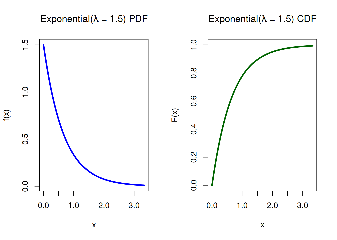
Example: A machine in a manufacturing plant occasionally breaks down. The time (in hours) between breakdowns follows an Exponential distribution with rate \(\lambda =1.5\). What is the probability that the machine runs for more than 1 hour before the next breakdown?
Customers arrive at a small service kiosk according to a Poisson process with rate \(\lambda =1.5\) customers per hour. That means:
The number of arrivals in time \(t\) is \(N(t)\sim \mathrm{Poisson}(\lambda t)\).
The waiting time between arrivals is \(X\sim \mathrm{Exponential}(\lambda )\).
What is the probability that the next customer arrives within 30 minutes (interarrival-time; exponential)?
pexp(q =0.5, rate =1.5)
[1] 0.5276334
What is the probability that exactly 2 customers arrive in the next hour (count; poisson)?
dpois(x =2, lambda =1.5)
[1] 0.2510214
6.2.3 Gamma Distribution
The gamma distribution generalises the exponential distribution. It represents the sum of independent exponential random variables, and also waiting time until the \(\alpha\)-th event in a Poisson process.
Why it matters in simulation
Provides flexible modelling of positive, skewed data.
Used in reliability and survival analysis.
Appears as a conjugate prior in Bayesian inference.
Forms the basis of many hierarchical models.
The gamma distribution allows more realistic modelling of waiting times than the exponential, by relaxing the memoryless assumption.
Let
\[
X\sim \mathrm{Gamma}(\alpha ,\beta )
\]
where \(\alpha >0\) is the shape parameter and \(\beta >0\) is the rate parameter (so the scale is \(1/\beta\).)
where \(\gamma (\alpha ,\beta x)\) is the lower incomplete gamma function.
The expectation and variance are \[
\mathbb{E}[X]=\frac{\alpha }{\beta }, \qquad
\mathrm{Var}(X)=\frac{\alpha }{\beta ^2}.
\]
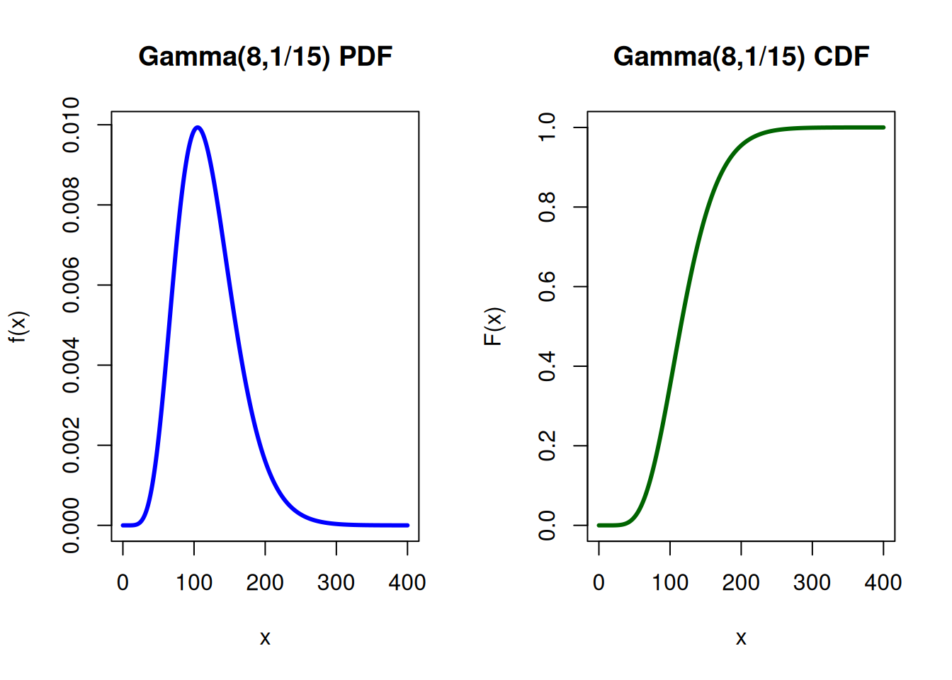
Example: Suppose a claim size X of a general insurance has gamma distribution with \(\alpha = 8\) and \(\beta = 1/15\). Calculate the probability that claim size is between 60 and 120.
s <-8 ; r <-1/15pgamma(q=120, shape=s, rate=r) -pgamma(q=60, shape=s, rate=r)
This is a beautiful link to the Poisson process — the Gamma(\(k\),\(\lambda\)) is the waiting time for the \(k\)‑th event.
Example: Customers arrive at a service counter according to a Poisson process with rate \(\lambda =2\) customers per hour. Let \(T_3\) be the waiting time until the 3rd customer arrives. Because the waiting time for the \(k\)-th event in a Poisson process is
What is the probability that the 3rd customer arrives within 2 hours?
pgamma(q =2, shape =3, rate =2)
[1] 0.7618967
6.2.4 Normal Distribution
The normal distribution or Gaussian distribution describes uncertainty as a symmetric bell-shaped curve. Arising through the Central Limit Theorem, it is considered the most important continuous distribution in applied probability.
What it matters in simulation
Many models assume normally distributed errors.
Gaussian random walks underlie MCMC algorithms.
Brownian motion is constructed from normal increments.
Variance estimation often relies on normal approximations.
Even when the true distribution is not normal, simulation output is often analysed using normal approximations.
The parameters \(\mu\) and \(\sigma^2\) represent the mean and variance.
Example A standardised test is designed so that student scores follow a standard normal distribution. If a student receives a z-score of 1.2 on the exam, what proportion of students scored below this student?
pnorm(1.2)
[1] 0.8849303
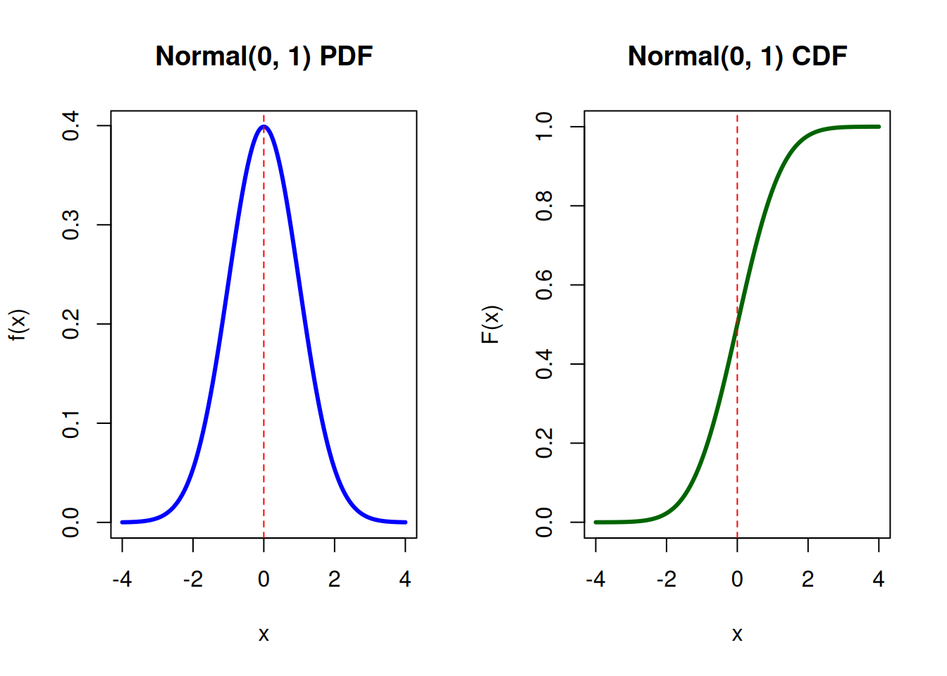
Standard Normal PMF and CDF
# Parametersmu <-0# meansigma <-1# standard deviation# Sequence of x values (cover most of the distribution)x <-seq(mu -4*sigma, mu +4*sigma, length =500)# PDF and CDFpdf <-dnorm(x, mean = mu, sd = sigma)cdf <-pnorm(x, mean = mu, sd = sigma)# Set plotting area: 1 row, 2 columnspar(mfrow =c(1, 2))# --- PDF Plot ---plot(x, pdf,type ="l",lwd =3,col ="blue",main ="Normal(0, 1) PDF",xlab ="x",ylab ="f(x)")abline(v = mu, lty =2, col ="red")# --- CDF Plot ---plot(x, cdf,type ="l",lwd =3,col ="darkgreen",main ="Normal(0, 1) CDF",xlab ="x",ylab ="F(x)",ylim =c(0, 1))abline(v = mu, lty =2, col ="red")
6.2.5 Log-Normal Distribution
The normal distribution is symmetric and defined over all real numbers, so it may not suit variables that are strictly positive or strongly skewed, such as body weight or stock prices. In such cases, distributions like the log‑normal are often more appropriate.
Why it matters in simulation
Used in financial modelling (asset prices).
Models service times with heavy right tails.
Arises naturally via transformation methods.
Demonstrates how distributions can be constructed via nonlinear transformation.
It is an important example of how tail behaviour changes under transformation.
Let \[
X\sim \mathrm{Lognormal}(\mu ,\sigma ^2)
\]
meaning
\[\ln X\sim N(\mu ,\sigma ^2).\]
The PDF is given by \[
f(x)=\frac{1}{x\sigma \sqrt{2\pi }}\exp \! \left( -\frac{(\ln x-\mu )^2}{2\sigma ^2}\right) ,\qquad x>0.
\]
The CDF is given by \[
F(x)=P(X\leq x)=\Phi \! \left( \frac{\ln x-\mu }{\sigma }\right) ,\qquad x>0,
\]
where \(\Phi (\cdot )\) is the standard normal CDF.
Then, the mean and variance are \[
\mathbb{E}[X]=e^{\mu +\frac{1}{2}\sigma ^2}, \qquad \mathrm{Var}(X)=\left( e^{\sigma ^2}-1\right) e^{2\mu +\sigma ^2}.\]
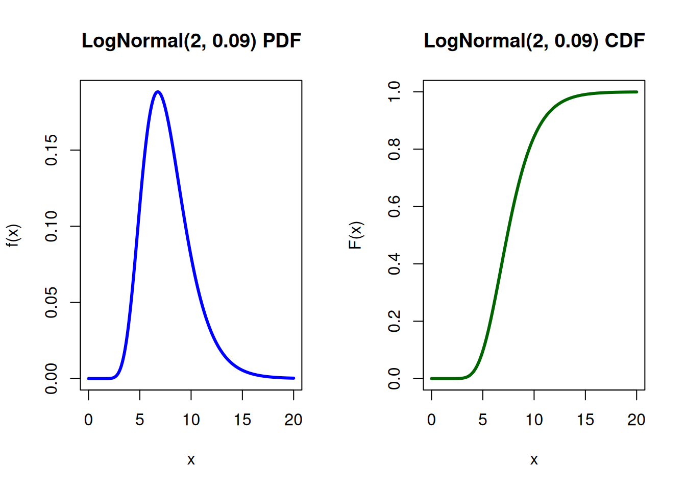
Example: the price of a certain stock is modeled as log‑normally distributed with parameters \(\mu =2\) and \(\sigma =0.3\). This means
\[
\ln (X)\sim N(2,\, 0.3^2).\]
What is the probability that the stock price is less than 10?
The beta distribution is defined on (0,1), making it ideal for modelling probabilities and proportions. In Bayesian inference, the beta distribution is the conjugate prior probability distribution for the Bernoulli, binomial, negative binomial, and geometric distributions. It has flexible shapes (U-shaped, symmetric, skewed).
Why it matters in simulation
Used in Bayesian updating.
Models uncertainty about probabilities.
Appears in hierarchical simulation models.
Useful in sensitivity analysis.
The beta distribution provides controlled randomness on a finite interval.
Let
\[
X\sim \mathrm{Beta}(\alpha ,\beta )
\]
with shape parameters \(\alpha >0\) and \(\beta >0\). The support is the interval \(0<x<1\).
where \(I_x(\alpha ,\beta )\) is the regularised incomplete beta function.
The mean and variance are \[
\mathbb{E}[X]=\frac{\alpha }{\alpha +\beta }, \qquad
\mathrm{Var}(X)=\frac{\alpha \beta }{(\alpha +\beta )^2(\alpha +\beta +1)}.
\]
Example: A website tracks the proportion of visitors who click on a new advertisement. Based on past data, the marketing team models the click‑through rate \(p\) as:
R provides a consistent and elegant naming convention for working with probability distributions. For nearly every standard distribution, four core functions are available. These functions allow us to compute probabilities, evaluate densities, calculate quantiles, and generate random samples.
The naming structure follows the pattern:
prefix + distribution
where the prefix determines the type of calculation being performed.
The four prefixes are:
d — density or mass function
p — cumulative distribution function
q — quantile function (inverse CDF)
r — random number generation
This systematic structure makes R particularly powerful for simulation work, since generating random variables, evaluating probabilities, and computing theoretical quantities all use parallel syntax.
For example, for the Normal distribution:
dnorm() evaluates the density
pnorm() evaluates the CDF
qnorm() computes quantiles
rnorm() generates random samples
This pattern is consistent across nearly all commonly used distributions.