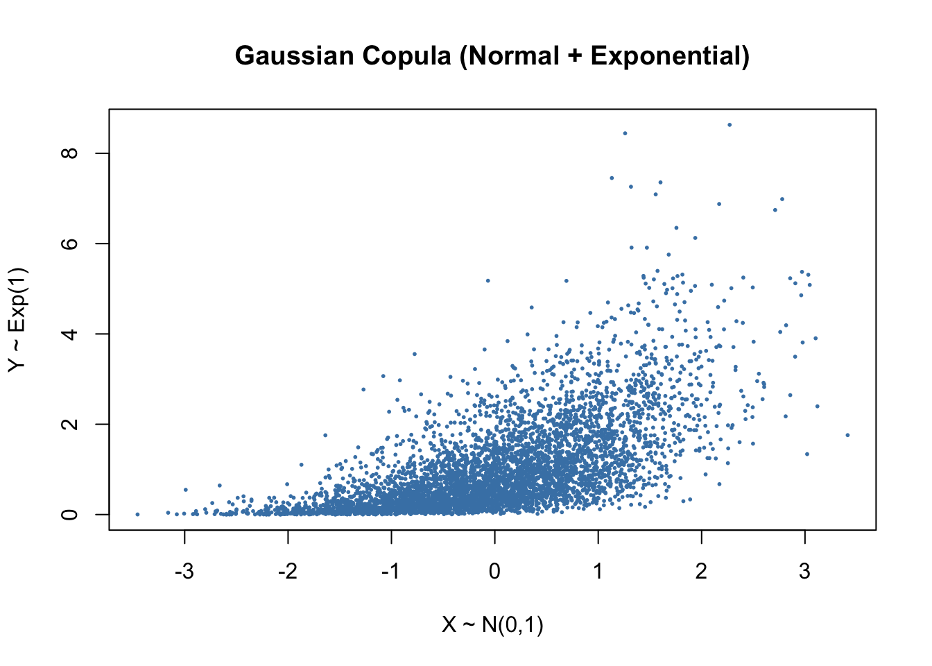
So far, we have constructed dependence using linear transformations of normal variables. This approach is powerful, but it has an important limitation:
It ties dependence to normality.
In many real-world applications (finance, insurance, environmental modelling), dependence can be:
non-linear,
asymmetric,
or stronger in extremes (tail dependence).
To model such behaviour, we need a more flexible framework.
This leads to the idea of copulas.
24.1 Copula
A copula is a function that allows us to construct a joint distribution by combining:
marginal distributions, and
a dependence structure.
Key Idea
Any joint distribution can be decomposed as:
\[
F_{X,Y}(x,y) = C\big(F_X(x), F_Y(y)\big),
\]
where:
\(F_X, F_Y\) are marginal CDFs,
\(C(u,v)\) is a copula.
This result is known as Sklar’s Theorem.
Interpretation
Marginals describe individual behaviour.
The copula describes dependence.
In copula models, dependence is often measured using:
Pearson correlation (linear)
Spearman’s rho (rank-based)
Kendall’s tau
Copulas naturally capture rank dependence, not just linear relationships.
Why Copulas Matter in Simulation
Copulas allow us to:
simulate dependence without assuming normality,
combine any marginal distributions (e.g., Normal + Exponential),
model tail dependence (important in risk modelling),
separate modelling into marginals (easy) or dependence (flexible).
Gaussian Copula
The most commonly used copula in simulation is the Gaussian copula.