18  Acceptance-Rejection Method

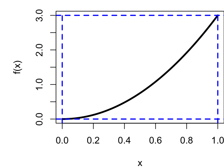
In the previous section, we saw that inverse transform sampling provides a direct and elegant way to generate random variables from a given distribution. However, this approach relies on the ability to compute and invert the cumulative distribution function (CDF), which is not always feasible in practice.

For many important distributions, the CDF:

• does not have a closed-form expression, or
• cannot be easily inverted numerically.

This limitation motivates the need for more flexible simulation techniques.

The acceptance–rejection method is a general approach that allows us to generate samples from a target distribution by using a simpler, easier-to-simulate distribution.

The key idea is:

Important

Instead of sampling directly from the target distribution, we generate candidate samples from a convenient distribution and accept or reject them with a carefully chosen probability.

More concretely, suppose we want to simulate a random variable with density \(f(x)\), but direct sampling is difficult. We instead:

1. Choose a proposal distribution g(x) that is easy to simulate from,
2. Ensure that \(f(x)\) is bounded by a multiple of g(x), i.e. \(f(x) \leq M g(x) \;\forall x\), where \(M > 0\) is a constant,
3. Generate a candidate value from g(x), and
4. Accept it with probability proportional to how well it matches \(f(x)\).

If the candidate is rejected, we simply try again.

This procedure produces samples that follow the target distribution \(f(x)\), even though we never sample from it directly. Intuitively, the method works by:

• oversampling from a simple distribution, and
• filtering those samples to match the desired shape.

The acceptance–rejection method is powerful because: - it applies to a wide range of distributions, - it does not require inverting the CDF, and - it forms the foundation for many advanced simulation algorithms.

However, its efficiency depends on how well the proposal distribution g(x) approximates the target distribution \(f(x)\). Poor choices can lead to many rejections and slow performance.

---

Motivation Example

We want to simulate from the density \[ f(x) = 3x^2, \quad 0 \le x \le 1. \]

First, verify this is a valid PDF: \[ \int_0^1 3x^2 \, dx = 1. \]

Although the CDF can be derived, inversion is not always convenient. Instead, we take a different approach.

Rather than transforming variables, we:

sample random points in a region and keep those that fall under the curve.

Consider the rectangle: \[ 0 \le x \le 1, \quad 0 \le y \le 3. \]

The curve \(y = 3x^2\) lies entirely inside this rectangle.

x <- seq(0, 1, length.out=100)
par(mar=c(4,5,1,0))
curve(3 * x^2, type = "l", lwd = 3, ylab = "f(x)")
abline(v=c(0,1), lwd = 2, lty = 2, col = "blue")
abline(h=c(0,3), lwd = 2, lty = 2, col = "blue")

• Points are generated uniformly in the rectangle
  
• Points below the curve are accepted
  
• Points above the curve are rejected

To simulate from \(f(x) = 3x^2\):

1. Generate:

   • \(X \sim \text{Uniform}(0,1)\)
   • \(Y \sim \text{Uniform}(0,3)\)

2. If \[ Y \le 3X^2, \] accept$ X$

3. Otherwise, reject and repeat

set.seed(123)
x <- runif(2000)
y <- runif(2000, 0, 3)

plot(x, y, pch = 16,
     col = ifelse(y <= 3*x^2, "blue", "red"),
     xlab = "x", ylab = "y",
     main = "Acceptance-Rejection Sampling")

curve(3*x^2, add = TRUE, col = "black", lwd = 3)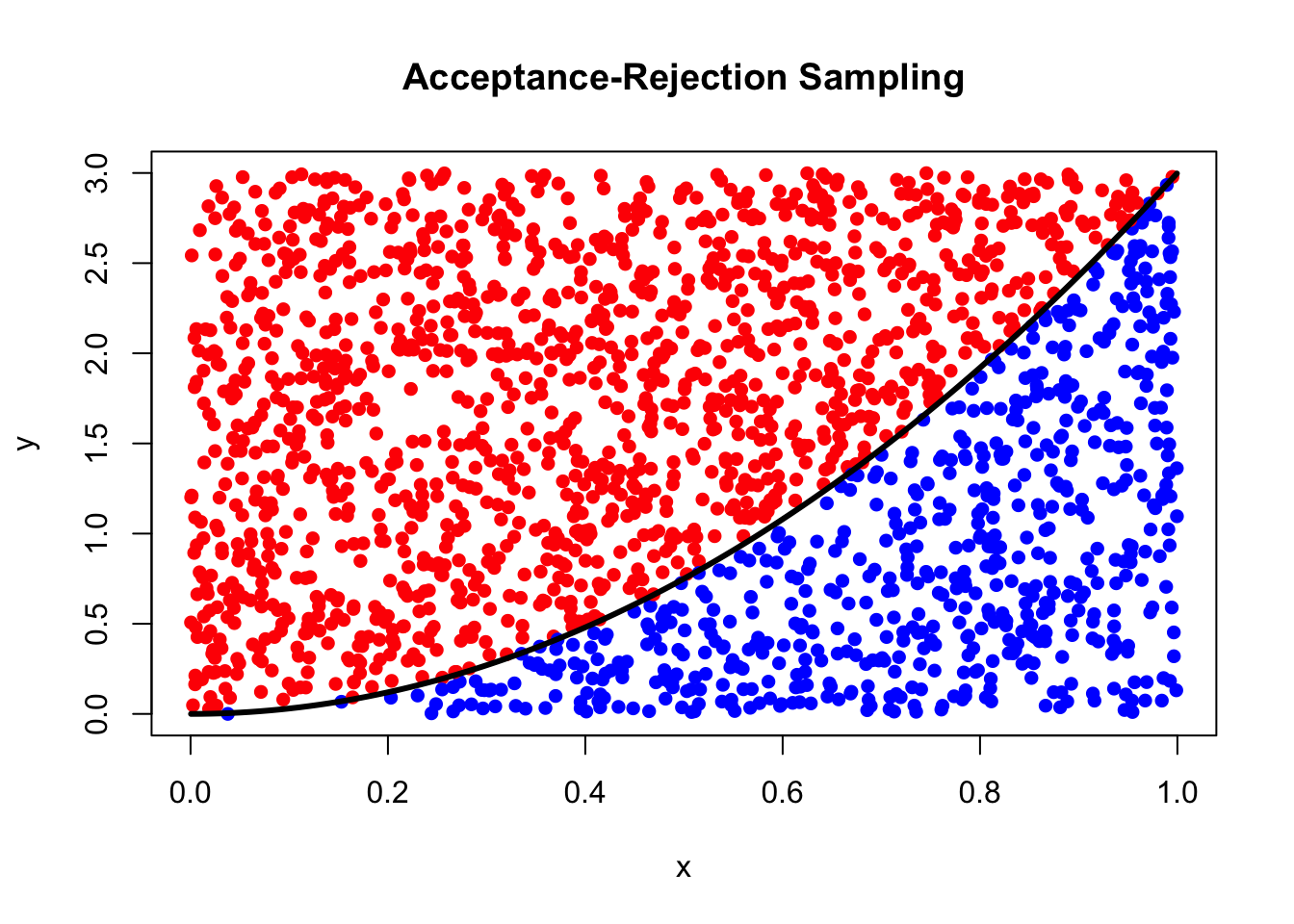

set.seed(1234)

n <- 10000

accepted <- numeric(0) # initialise numeric variables/vectors

while(length(accepted) < n){ # keep sampling until we have n accepted values
  x <- runif(1) # proposal: X ~ Uniform(0,1)
  y <- runif(1, 0, 3) # auxiliary variable: Y ~ Uniform(0, 3)
  
  if(y <= 3 * x^2){ # accept if point lies under the curve f(x)
    accepted <- c(accepted, x) # keep accepted x
  } # otherwise reject and try again
}

hist(accepted, prob = TRUE, col = "skyblue", main = "Acceptance-Rejection Sampling")
lines(density(accepted), col = "blue", lwd = 2) # Kernel Density Estimate (KDE)
curve(3 * x^2, col = "red", lwd = 2, add = TRUE) # True Density

legend("topleft", legend = c("Histogram", "KDE", "True density"),
       col = c("skyblue", "blue", "red"),
       lwd = c(NA, 2, 2), pch = c(15, NA, NA), bty = "n")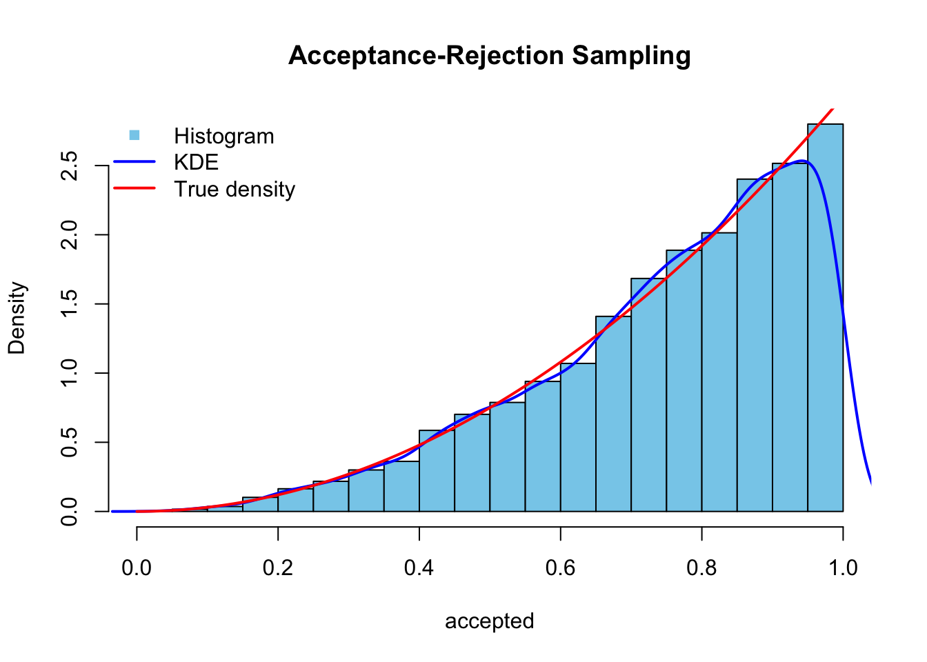

General Algorithm

The rectangular approach works well when:

• the support is simple,
• the density is bounded,
• and a rectangle is easy to construct.

However, many distributions are more complex. We therefore generalise the idea.

Suppose we want to simulate from a target density \(f(x)\).

Choose:

• a proposal density \(g(x)\),
• a constant \(M > 0\),

such that \[ f(x) \le M g(x) \quad \forall x. \]

Then \(Mg(x)\) acts as an envelope over \(f(x)\).

To simulate \(X \sim f(x):\)

1. Generate \(Y \sim g(x)\)

2. Generate \(U \sim \text{Uniform}(0,1)\)

3. Accept \(Y\) if \[ U \le \frac{f(Y)}{M g(Y)} \]

4. Otherwise, reject and repeat

If accepted, set \(X = Y\).

Efficiency of the Method

The probability of acceptance is: \[ \frac{1}{M}. \]

• smaller \(M\) → higher efficiency
• larger \(M\) → more rejections

---

Cubic Polynomial CDF Example

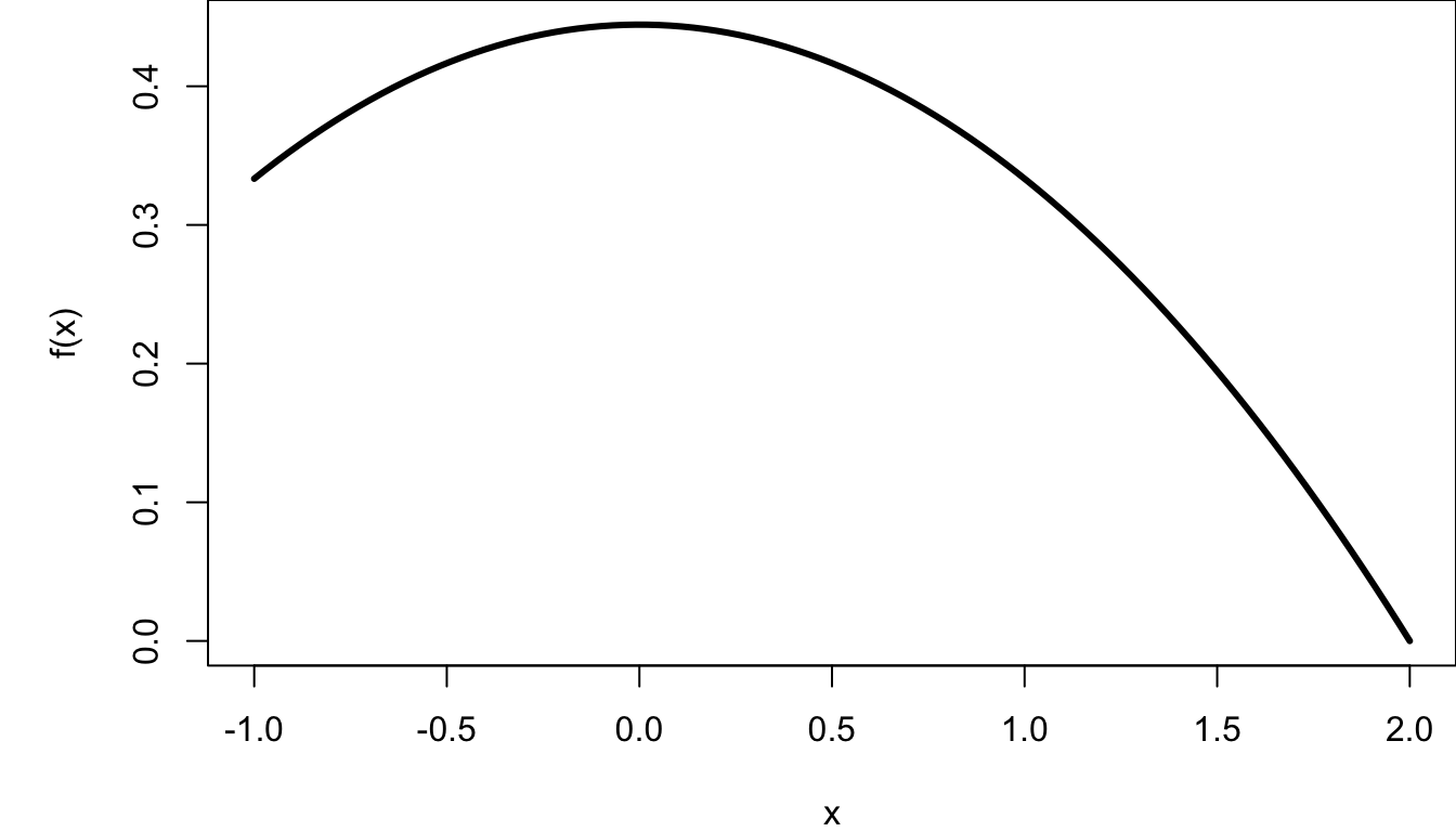
The measurement error \(X\) (in mV) of a particular volt-meter has the following distribution:

\[ f(x) = \begin{cases} \dfrac{4-x^2}{9}, & \quad -1 \leq x \leq 2 \\ 0, & \text{otherwise.} \end{cases} \]

Simulate \(f(x)\) using acceptance-rejection method.

Step 0: Check whether \(f(x)\) is valid

\[ \int_{-1}^2 \frac{4-x^2}{9} \,dx = 1 \rightarrow \text{ valid PDF.} \]

Step 1: Determine \(Mg(x); f(x) \leq Mg(x)\)

Because the support is bounded, the best first proposal is:

\[ g(x) = \text{Uniform}(-1, 2) = \frac{1}{3}, \quad -1 \leq x \leq 2. \]

Since \(g(x)=1/3\), this becomes

\[ \frac{4-x^2}{3} \leq M \]

Now on [-1, 2], the maximum of LHS occurs at \(x=0,\)

\[ \max_{-1\leq x \leq 2} \frac{4-x^2}{3} = \frac{4}{3} \]

Hence, we can choose

\[ M = \frac{4}{3} \quad \text{ with an acceptance rate of } \quad \frac{1}{M} = \frac{3}{4} = 75\% \]

This gives

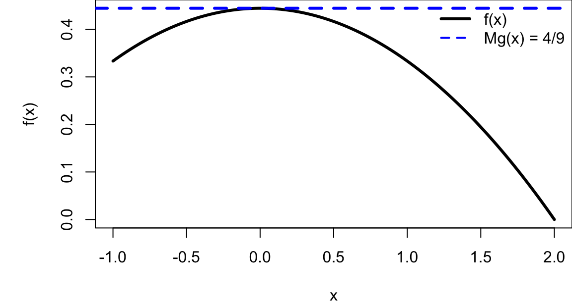
\[ Mg(x) = \frac{4}{3} \cdot \frac{1}{3} = \frac{4}{9} \]

So the envelope is just a horizontal line at height 4/9.

---

Step 2: Determine the acceptance rule

The general rule is

\[ U \leq \frac{f(Y)}{Mg(Y)} \]

where \(Y\sim g\) and \(U \sim \text{Uniform}(0,1).\)

Substitute in, gives

\[ \frac{f(Y)}{Mg(Y)} = \frac{4-y^2}{4} \]

So accept \(Y\) if

\[ U \leq \frac{4-y^2}{4}. \]

set.seed(1234)
n <- 10000
x <- numeric(0) # store accepted samples

while(length(x) < n){ # keep sampling until we have n accepted values
  y <- runif(n, min = -1, max = 2)   # proposal sample Y ~ g(x) ~ Uniform(-1, 2)
  u <- runif(n)                      # U ~ Uniform(0,1) for acceptance test
  accept <- u <= (4 - y^2)/4         # acceptance rule (returns TRUE/FALSE)
  x <- c(x, y[accept])               # keep accepted y
}

x <- x[1:n] # trim to exactly n samples

hist(x, prob = TRUE, breaks = 40,
     col = "lightgray", border = "white",
     main = "Acceptance-Rejection Sampling",
     xlab = "x")

curve((4 - x^2)/9, from = -1, to = 2,
      add = TRUE, col = "red", lwd = 2)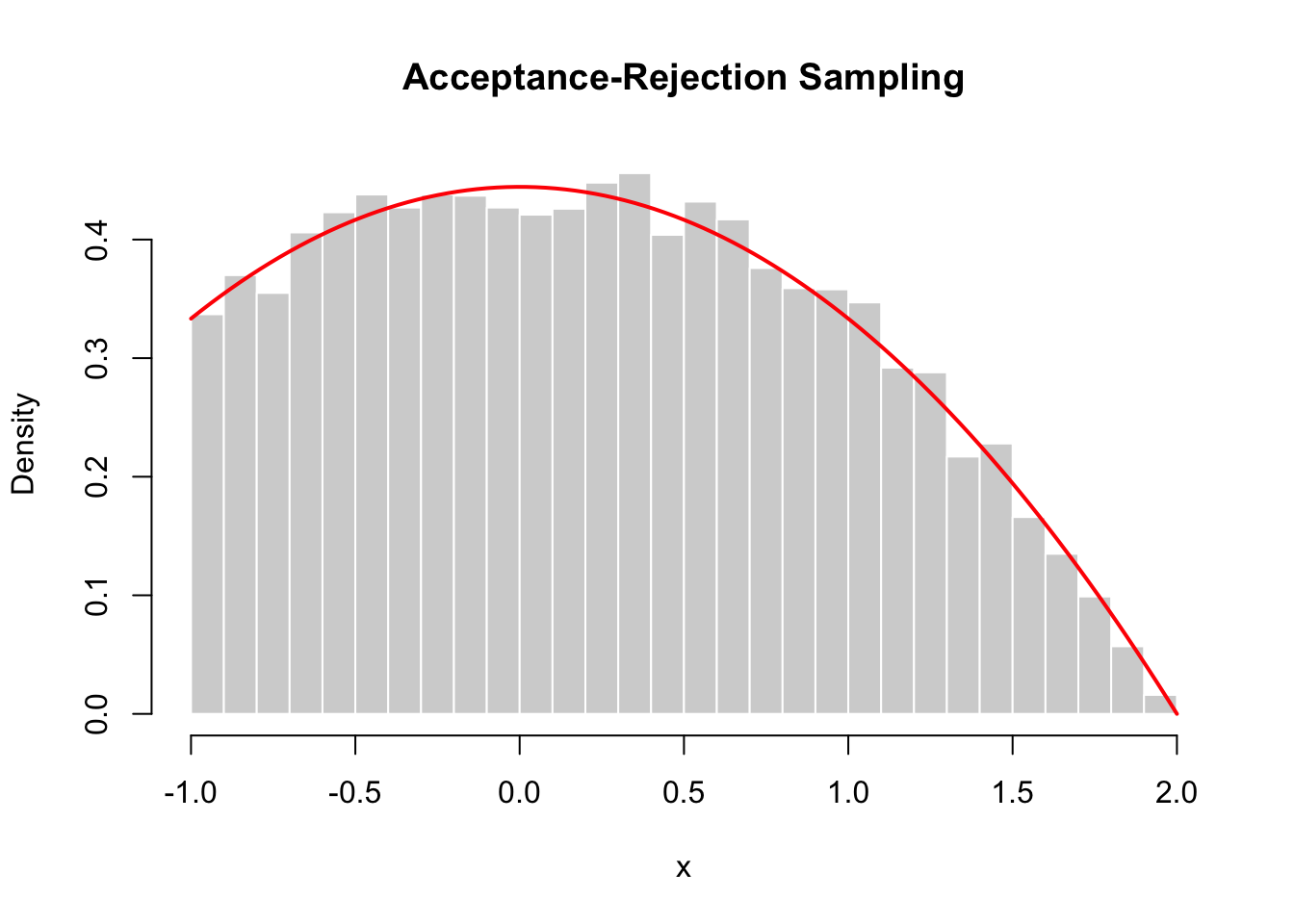

---

Normal-Cauchy Example

Generate the standard normal distribution using the standard Cauchy distribution

Recall the PDF of \(X \sim N(0, 1):\)

\[ f(x)=\frac{1}{\sqrt{2\pi}}\exp{\left(-\frac{x^2}{2}\right)}, \quad x \in \mathbb{R}. \]

The PDF of \(X \sim \text{Cauchy}:\)

\[ g(x) = \frac{1}{\pi(1+x^2)}, \quad x \in \mathbb{R}. \]

Let’s compare the distributions:

x <- seq(-5, 5, length = 200)
dc <- dcauchy(x, location = 0, scale = 1)
dn <- dnorm(x, mean = 0, sd = 1)

par(mfrow=c(1,2), mar=c(4,5,1,1))
plot(x, dn, type="l", ylab="Density")
lines(x, dc, col="blue", lty=2)
legend("topright", col=c("black", "blue"), lty=c(1,2),
       legend =c("Normal", "Cauchy"), ncol=2, bty = "n" )
plot(x, dn/dc, type="l", ylab="f(x) / g(x)")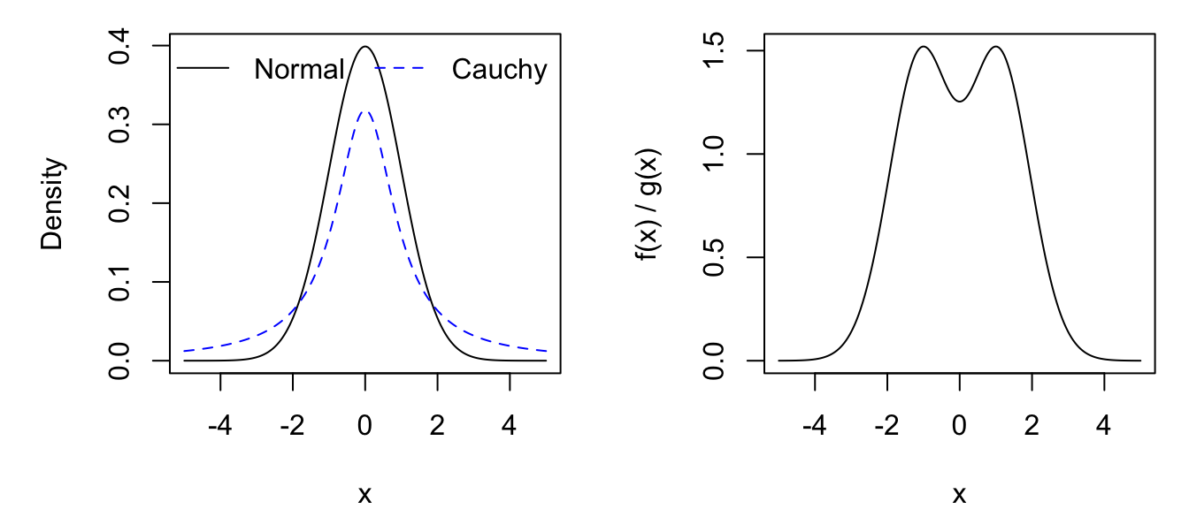

• From RHS, the standard cauchy distribution is wider but shorter than the standard normal distribution.
• From LHS, the \(f(x)/g(x)\) ratio is maximised around 1.5.

Step 1: Find \(M\)

\[ \frac{f(x)}{g(x)} = \frac{1}{\sqrt{2\pi}}\exp{\left(-\frac{x^2}{2}\right)} \cdot \pi(1+x^2) = \frac{\pi}{\sqrt{2\pi}}(1+x^2)\exp{\left(-\frac{x^2}{2}\right)} \]

\[ \max_{-\infty < x < \infty}{(1+x^2)\exp{\left(-\frac{x^2}{2}\right)}} \]

Differentiate and set it equal to 0:

\[ \begin{aligned} \frac{d}{dx} \left(\frac{f(x)}{g(x)}\right) &= 2x\exp{\left(-\frac{x^2}{2}\right)} + (1+x^2)(-x)\exp{\left(-\frac{x^2}{2}\right)} \\ 0 &= \exp{\left(-\frac{x^2}{2}\right)} x (1-x^2) \end{aligned} \]

yields three critical points: \(x = 0, x = \pm 1.\)

• From the ratio plot, we would expect the maximum to occur at \(x = \pm 1.\)

• If this is not obvious, use the second derivative test to verify.

Substitute \(x= \pm 1\) into \(f(x)/g(x)\) yields

\[ M=2e^{-1/2}\sqrt{\frac{\pi}{2}}\approx 1.5203 \rightarrow \text{ with the acceptance probability of } 0.6577. \]

Step 2: Determine the acceptance rule

The general rule is

\[ U \leq \frac{f(Y)}{Mg(Y)} \]

where \(Y\sim g \sim \text{Cauchy}\) and \(U \sim \text{Uniform}(0,1).\)

Substitute in, gives the acceptance rule

\[ U \leq \frac{f(Y)}{Mg(Y)} = \frac{\sqrt{e}}{2} (1+y^2) \exp{\left(-\frac{y^2}{2}\right)} \]

set.seed(1234)
n <- 5000              # number of samples needed
M <- 2 * exp(-1/2) * sqrt(pi/2)   # exact M ≈ 1.5203
samples <- numeric(0)

while(length(samples) < n){
  y <- rcauchy(n) # propose from Cauchy
  u <- runif(n)   # uniform for acceptance
  f <- dnorm(y)   # target density
  g <- dcauchy(y) # proposal density
  
  accept <- u <= f / (M * g) # acceptance rule
  samples <- c(samples, y[accept])  # keep accepted values
}

samples <- samples[1:n] # trim to exactly n samples

hist(samples, prob = TRUE, breaks = 40,
     col = "lightgray",
     main = "Normal via Acceptance-Rejection (Cauchy proposal)",
     xlab = "x")

curve(dnorm(x), add = TRUE, col = "red", lwd = 2)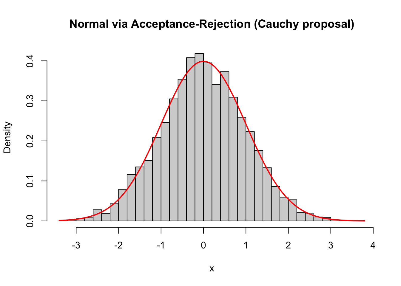

set.seed(1234)
y <- rcauchy(5000); u <- runif(5000)
M <- 2 * exp(-1/2) * sqrt(pi/2)
accept <- u <= dnorm(y) / (M * dcauchy(y))
cat("The empirical acceptance rate is", mean(accept))

The empirical acceptance rate is 0.6578