In many applications, we work not with a single random variable but with a pair (or vector) of variables whose joint distribution is known. When we apply a transformation to such a pair, the result is a new pair of random variables whose joint distribution we often need to determine. This section develops the tools for understanding how probability densities change under transformations of two (or more) variables.
Transformations of multiple random variables arise naturally in statistics, simulation, and modelling. Examples include converting Cartesian coordinates to polar coordinates, forming sums and differences of random variables, and applying linear transformations to generate correlated normals. The key idea is that probability must be preserved under the transformation, and the mathematical tool that ensures this is the Jacobian.
22.1 Transformations of Two Random Variables
Why This Matters
Transformations of multiple random variables allow us to:
derive distributions of sums, ratios, and other combinations,
change coordinate systems to simplify integrals,
understand how linear maps create covariance,
simulate multivariate distributions efficiently,
and prepare for higher‑dimensional transformations in later topics.
This section builds the foundation for the next major topic: linear transformations and the multivariate normal, where the Jacobian plays a central role in understanding how densities behave under matrix transformations.
Suppose \((X, Y)\) has a known joint density \(f_{X,Y}(x,y)\), and we define a new pair:
\[
U = g_1(X, Y), \qquad V = g_2(X, Y).
\]
Our goal is to find the joint density \(f_{U,V}(u,v)\).
If the transformation is one‑to‑one and differentiable, we can invert it:
\[
x = h_1(u,v), \qquad y = h_2(u,v),
\]
and use the Jacobian determinant to adjust for how the transformation stretches or compresses area.
22.2 The Jacobian Formula (Continuous Case)
If the transformation is smooth and invertible, then
is the Jacobian matrix of the inverse transformation.
The determinant \(|\det J|\) measures how the transformation changes area, ensuring that total probability remains 1.
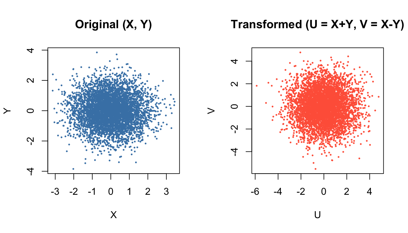
Example 1: Sums and Differences
Let \((X,Y)\) have joint density \(f_{X,Y}(x,y)\). Defin
\[
U = X + Y, \qquad V = X - Y.
\]
This transformation is linear and invertible, and the Jacobian is constant.
It is widely used in deriving distributions of sums of independent normals.
Step 1: Invert the transformation
Solve for \(X, Y\) in terms of \(U, V\):
\[
X = \dfrac{U + V}{2}, \qquad Y = \dfrac{U - V}{2}.
\]
So
\[
x = h_1(u,v) = \dfrac{u+v}{2}, \quad
y = h_2(u,v) = \dfrac{u-v}{2}.
\]
\[
f_{R,\Theta}(r,\theta)
= f_{X,Y}(r\cos\theta, r\sin\theta)\cdot r.
\]
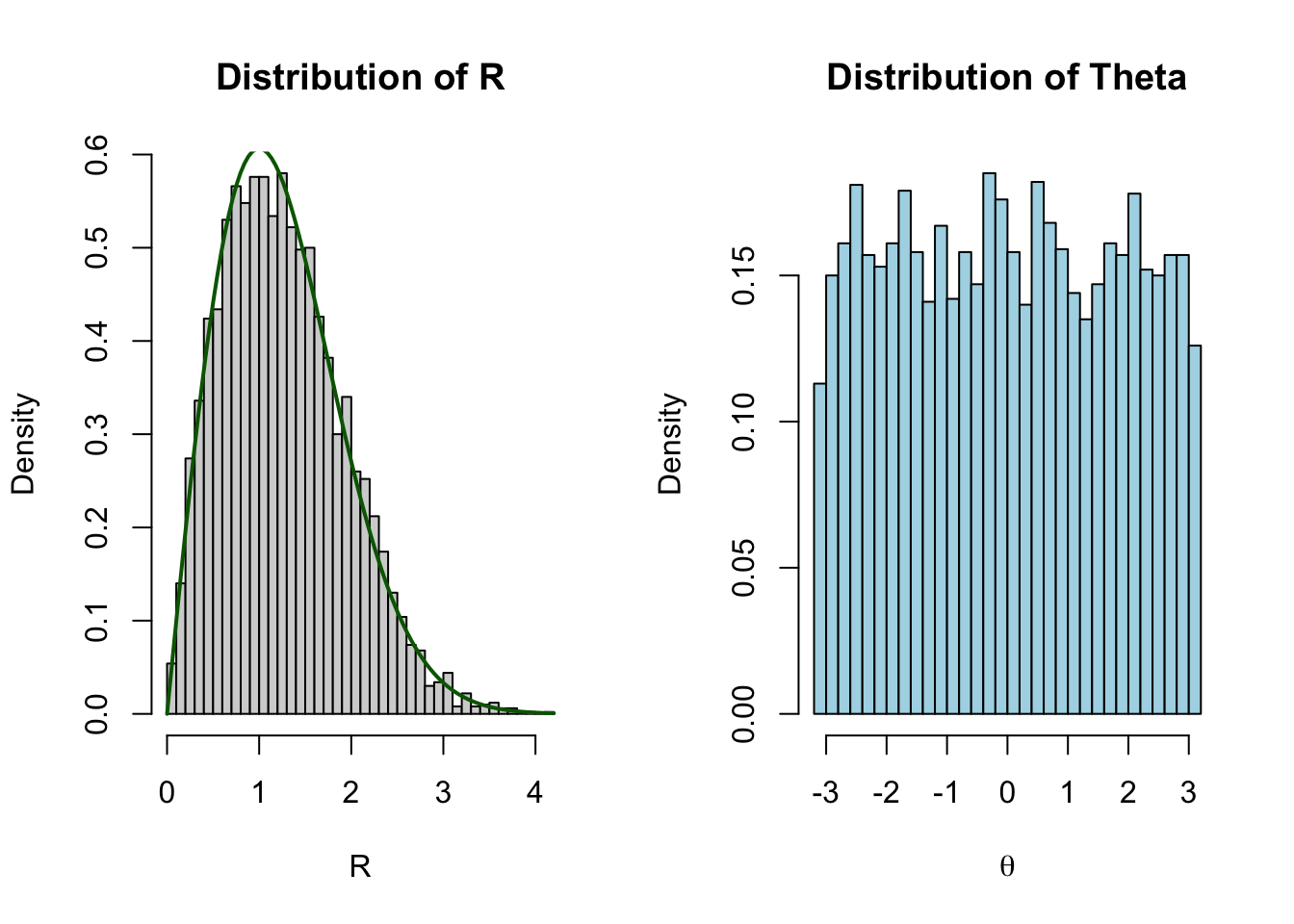
set.seed(1)n <-5000X <-rnorm(n)Y <-rnorm(n)R <-sqrt(X^2+ Y^2)Theta <-atan2(Y, X)par(mfrow =c(1, 2))hist(R, breaks =40, freq =FALSE, col ="lightgray",main ="Distribution of R",xlab ="R")curve(dchisq(x^2, df =2) *2*x, add =TRUE, col ="darkgreen", lwd =2)hist(Theta, breaks =40, freq =FALSE, col ="lightblue",main ="Distribution of Theta",xlab =expression(theta))
R follows the Rayleigh distribution (equivalently, \(R^2\sim \chi_2^2\)).
\(\Theta\) is uniform on \([-\pi ,\pi ]\).
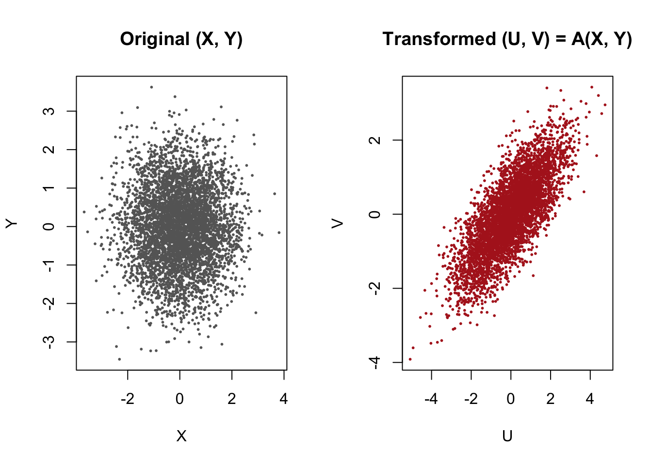
Example 3: Linear Transformations
Let \((X, Y)\) have joint density \(f_{X,Y}(x,y)\), and let \[
\begin{pmatrix} U \\ V \end{pmatrix}
=
A \begin{pmatrix} X \\ Y \end{pmatrix},
\quad
A =
\begin{pmatrix}
a & b \\
c & d
\end{pmatrix},
\]
with \(\det A \neq 0\). Then the Jacobian determinant is simply \(|\det A|\).
This case is especially important for the multivariate normal distribution, where linear transformations create covariance structures. The correlated‑normal simulation you used earlier is a special case of this idea.
Step 1: Invert the transformation
Because \(\det A \neq 0\), \(A\) is invertible:
\[
\begin{pmatrix} X \\ Y \end{pmatrix}
= A^{-1} \begin{pmatrix} U \\ V \end{pmatrix}.
\]
Write
\[
A^{-1} =
\frac{1}{ad - bc}
\begin{pmatrix}
d & -b \\
-c & a
\end{pmatrix}.
\]
So
\[
x = h_1(u,v), \quad y = h_2(u,v)
\]
are linear functions of \((u,v)\).
Step 2: Jacobian of the inverse
For a linear map, the Jacobian matrix of the inverse is just \(A^{-1}\), so