import numpy as np
from scipy.stats import geom
import matplotlib.pyplot as plt

np.random.seed(123)

n = 10000
p = 0.3

# scipy.stats.geom uses support {1,2,3,...} for "trial of first success"
# So subtract 1 to match R's convention (number of failures).
x = geom.rvs(p, size=n) - 110 Python Workshop Solutions
This workshop consists of two parts:
- Part 1: Univariate distributions in simulation
- Part 2: Joint distributions and dependence
Key scipy.stats Functions for Univariate Distributions
In Python, a package scipy.stats provides the probability‑distribution machinery, and matplotlib provides the plotting layer, so together they let you both generate random variables from any univariate distribution and visualise their empirical behaviour against theoretical curves.
With scipy.stats, each distribution comes with methods for simulation (.rvs()), probability mass/density evaluation (.pmf(), .pdf()), and cumulative or survival functions (.cdf(), .sf()), which makes it easy to reproduce the same workflows you would do in R.
| Distribution | PMF/PDF Function | CDF Function | Random Generation (rvs) |
Notes |
|---|---|---|---|---|
| Bernoulli | bernoulli.pmf(x, p) |
bernoulli.cdf(x, p) |
bernoulli.rvs(p, size=n) |
Support {0,1} |
| Binomial | binom.pmf(x, n, p) |
binom.cdf(x, n, p) |
binom.rvs(n, p, size=n) |
Number of successes in n trials |
| Geometric | geom.pmf(x, p) |
geom.cdf(x, p) |
geom.rvs(p, size=n) |
SciPy uses support {1,2,…}; subtract 1 for “failures before success” |
| Negative Binomial | nbinom.pmf(x, r, p) |
nbinom.cdf(x, r, p) |
nbinom.rvs(r, p, size=n) |
Counts failures before r successes |
| Poisson | poisson.pmf(x, λ) |
poisson.cdf(x, λ) |
poisson.rvs(λ, size=n) |
Mean = variance = λ |
| Multinomial | multinomial.pmf(x, n, p) |
No closed-form CDF | multinomial.rvs(n, p, size=k) |
Vector-valued counts |
| Uniform | uniform.pdf(x, loc, scale) |
uniform.cdf(x, loc, scale) |
uniform.rvs(loc, scale, size=n) |
On interval ([loc, loc+scale]) |
| Exponential | expon.pdf(x, scale=1/λ) |
expon.cdf(x, scale=1/λ) |
expon.rvs(scale=1/λ, size=n) |
Memoryless continuous distribution |
| Gamma | gamma.pdf(x, a, scale) |
gamma.cdf(x, a, scale) |
gamma.rvs(a, scale, size=n) |
Shape a, scale θ |
| Normal | norm.pdf(x, μ, σ) |
norm.cdf(x, μ, σ) |
norm.rvs(μ, σ, size=n) |
Gaussian distribution |
| Log-normal | lognorm.pdf(x, s, scale) |
lognorm.cdf(x, s, scale) |
lognorm.rvs(s, scale, size=n) |
s = σ of underlying normal |
| Beta | beta.pdf(x, a, b) |
beta.cdf(x, a, b) |
beta.rvs(a, b, size=n) |
Support on (0,1) |
Once you generate samples, matplotlib handles the visualisation: bar plots for discrete PMFs, histograms for continuous densities, and line plots for overlaying theoretical curves. This combination mirrors the R workflow closely—scipy.stats plays the role of rgeom, dgeom, etc., while matplotlib plays the role of barplot, plot, and hist—and gives you a consistent, reproducible way to teach simulation, empirical vs theoretical comparison, and distributional intuition across all univariate distributions.
Caution
R and Python do not use the same pseudorandom number generator, even when you set the same seed. That means set.seed(123) in R and np.random.seed(123) in Python will not produce the same sequence of random draws.
Part 1: Univariate distributions in simulation
Exercise 1: Geometric Distribution
Let \[X \sim \text{Geometric}(p),\] where \(p = 0.3\).
- Simulate 10,000 observations.
- Plot the empirical PMF (barplot of relative frequencies).
- Overlay the theoretical PMF.
- Compute:
- empirical mean and variance
- theoretical mean and variance
- Explain:
- Why is the geometric distribution memoryless? Verify: \(P(X>s+t | X>s)=P(X>t)\)
- How does changing \(p\) affect skewness?
- Estimate \(P(X > 5)\) analytically and via simulation. Compare results.
Solution
- Simulate 10,000 observations.
- Plot the empirical PMF (barplot of relative frequencies).
- Overlay the theoretical PMF.
# empirical PMF
vals, counts = np.unique(x, return_counts=True)
emp_pmf = counts / n

# theoretical PMF for same x-range
theo_pmf = geom.pmf(vals + 1, p)  # +1 because scipy's geom starts at 1

plt.figure(figsize=(8,5))
plt.bar(vals, emp_pmf, color="skyblue", label="Empirical PMF")
plt.plot(vals, theo_pmf, "ro-", label="Theoretical PMF")
plt.xlabel("x (failures before first success)")
plt.ylabel("Probability")
plt.title("Geometric(p=0.3): Empirical vs Theoretical PMF")
plt.legend()
plt.show()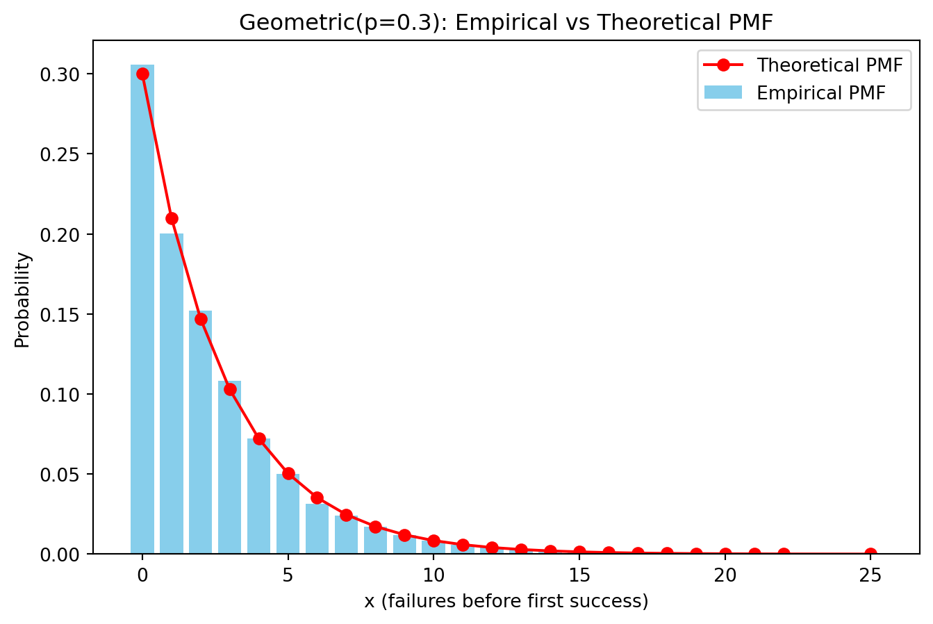
Empirical PMF closely matches theoretical PMF.
- Compute:
- empirical mean and variance
- theoretical mean and variance
# empirical
emp_mean = np.mean(x)
emp_var  = np.var(x, ddof=1)

# theoretical (R-style parameterization)
theo_mean = (1 - p) / p
theo_var  = (1 - p) / (p**2)

print("Empirical mean:", emp_mean)
print("Empirical variance:", emp_var)
print("Theoretical mean:", theo_mean)
print("Theoretical variance:", theo_var)
Empirical mean: 2.2958
Empirical variance: 7.378440204020402
Theoretical mean: 2.3333333333333335
Theoretical variance: 7.777777777777778- The reason empirical mean (and variance) are close to the theoretical values is due to the Law of Large Numbers (LLN).
- Variance closeness is also due to consistency (LLN applied to functions of X).
- Explain:
- Why is the geometric distribution memoryless? Verify: \(P(X>s+t | X>s)=P(X>t)\)
- How does changing \(p\) affect skewness?
Using conditional probability:
\[ P(X>s+t \mid X>s) = \frac{P(X>s+t)}{P(X>s)}, \]
and mean(x >= k) to estimate P(X>k)
s = 3
t = 4

lhs = np.mean(x >= (s + t)) / np.mean(x >= s)
rhs = np.mean(x >= t)

print("LHS (simulated):", lhs)
print("RHS (simulated):", rhs)
LHS (simulated): 0.23436586791350086
RHS (simulated): 0.234Mathematically, for a geometric distribution:
\[ P(X>k) = (1-p)^{k+1}, \]
So,
\[ \frac{P(X>s+t)}{P(X>s)} = \frac{(1-p)^{s+t+1}}{(1-p)^{s+1}} = (1-p)^t = P(X>t) \]
The cancellation is why memorylessness holds.
# Effect of changing p
ps = [0.3, 0.5, 0.7, 0.9]
colors = ["blue", "red", "purple", "green"]

plt.figure(figsize=(8,5))

for i, p_i in enumerate(ps):
    x_i = geom.rvs(p_i, size=n) - 1
    vals_i, counts_i = np.unique(x_i, return_counts=True)
    pmf_i = counts_i / n

    if i == 0:
        plt.plot(vals_i, pmf_i, "o-", color=colors[i], label=f"p={p_i}")
    else:
        plt.plot(vals_i, pmf_i, "o-", color=colors[i], label=f"p={p_i}")

plt.xlabel("x")
plt.ylabel("Relative frequency")
plt.title("Effect of p on Geometric Distribution Shape")
plt.legend()
plt.show()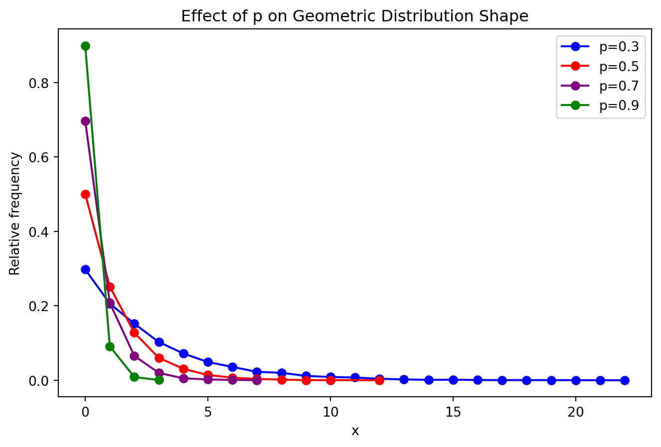
Increasing \(p\) makes the curve shift left and decay faster, concentrating more probability at small values (especially at 0).
- Estimate \(P(X > 5)\) analytically and via simulation. Compare results.
k = 5

analytic_prob = (1 - p)**(k + 1)
sim_prob = np.mean(x > k)

print("Analytic P(X>5):", analytic_prob)
print("Simulated P(X>5):", sim_prob)
Analytic P(X>5): 0.11764899999999996
Simulated P(X>5): 0.1115We are verifying that the simulated tail probability matches the theoretical geometric survival probability \(P(X>5) = (1-p)^{5+1} = 0.117649\).
Exercise 2: Gamma Distribution
Let \[X \sim \text{Gamma}(\alpha = 3, \beta = 2)\] (Use shape–rate parameterisation.)
- Simulate 10,000 observations.
- Plot histogram with theoretical density overlay.
- Compute empirical vs theoretical mean and variance.
- Investigate how changing \(\alpha\) affects:
- skewness
- tail behaviour
Solution
- Simulate 10,000 observations.
from scipy.stats import gamma

np.random.seed(123)

n = 10000
alpha = 3
beta = 2   # rate
scale = 1 / beta   # SciPy uses scale = 1/rate

x = gamma.rvs(a=alpha, scale=scale, size=n)- Plot histogram with theoretical density overlay.
plt.figure(figsize=(8,5))

# histogram as density
plt.hist(x, bins=40, density=True, alpha=0.6, edgecolor='black')

# theoretical density on same range
xs = np.linspace(0, x.max(), 500)
pdf_vals = gamma.pdf(xs, a=alpha, scale=scale)

plt.plot(xs, pdf_vals, 'r-', lw=2, label='Theoretical PDF')
plt.xlabel("x")
plt.ylabel("Density")
plt.title("Gamma(α=3, β=2): Empirical Histogram + Theoretical PDF")
plt.legend()
plt.show()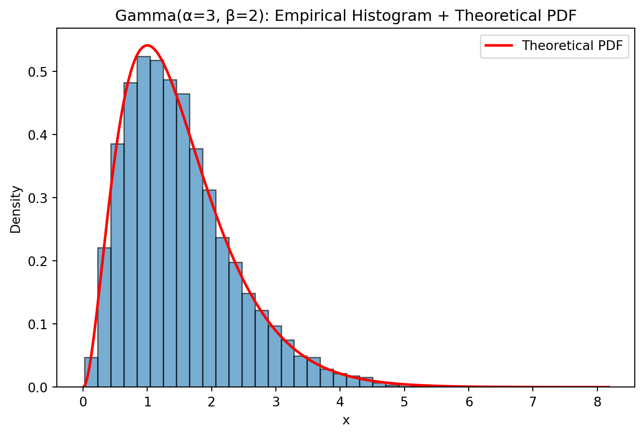
- Compute empirical vs theoretical mean and variance.
emp_mean = np.mean(x)
emp_var  = np.var(x, ddof=1)

theo_mean = alpha / beta
theo_var  = alpha / (beta**2)

print("Empirical mean:", emp_mean)
print("Theoretical mean:", theo_mean)
print("Empirical variance:", emp_var)
print("Theoretical variance:", theo_var)
Empirical mean: 1.5100165009253022
Theoretical mean: 1.5
Empirical variance: 0.7485340154615578
Theoretical variance: 0.75With large \(n\), the empirical values should be very close.
- Investigate how changing \(\alpha\) affects:
- skewness
- tail behaviour
np.random.seed(123)

alphas = [1, 2, 3, 5, 10]
beta = 2
scale = 1 / beta
n = 10000

# simulate samples for each alpha
samples = [gamma.rvs(a=a, scale=scale, size=n) for a in alphas]

# common x-grid for plotting
xmax = max(s.max() for s in samples)
xs = np.linspace(0, xmax, 1000)

plt.figure(figsize=(8,5))

for i, a in enumerate(alphas):
    pdf_vals = gamma.pdf(xs, a=a, scale=scale)
    plt.plot(xs, pdf_vals, lw=2, label=f"alpha = {a}")

plt.xlabel("x")
plt.ylabel("Density")
plt.title("Gamma PDFs for Different α (β fixed at 2)")
plt.legend()
plt.show()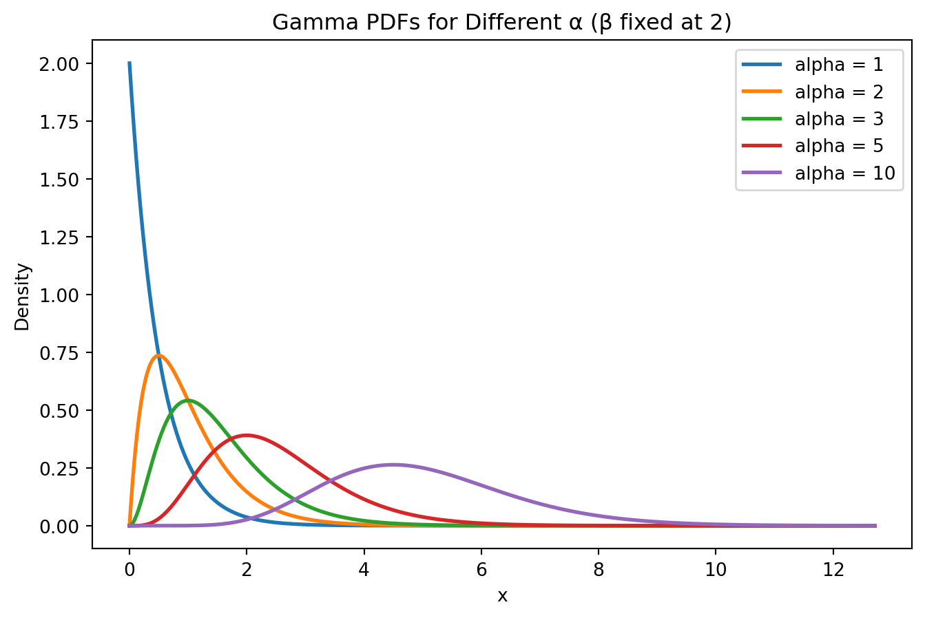
With \(\beta\) fixed, increasing \(\alpha\) has the following effects:
- Skewness decreases (more “bell-shaped”).
- Tail becomes less extreme relative to the center.
- The distribution concentrates more around its mean (and looks more normal-like), so very large values become less common relative to the bulk.
Exercise 3: Beta Distribution
Let \[X \sim \text{Beta}(2,5).\]
- Simulate 10,000 observations.
- Plot histogram and density.
- Compute mean and variance.
- Repeat for:
- Beta(0.5, 0.5)
- Beta(5, 5)
- How do the shape parameters affect:
- symmetry?
- concentration?
- boundary behaviour?
Solution
- Simulate 10,000 observations.
import numpy as np
import matplotlib.pyplot as plt
from scipy.stats import beta

np.random.seed(123)

n = 10000
a, b = 2, 5

x = beta.rvs(a, b, size=n)- Plot histogram and density.
plt.figure(figsize=(8,5))

# histogram as density
plt.hist(x, bins=30, density=True, alpha=0.6, edgecolor='black')

# theoretical density
xs = np.linspace(0, 1, 500)
pdf_vals = beta.pdf(xs, a, b)
plt.plot(xs, pdf_vals, 'r-', lw=2, label='Theoretical density')

# empirical density estimate
from scipy.stats import gaussian_kde
kde = gaussian_kde(x)
plt.plot(xs, kde(xs), 'b--', lw=2, label='Empirical density')

plt.xlabel("x")
plt.ylabel("Density")
plt.title("Beta(2,5): Histogram + Density")
plt.legend()
plt.show()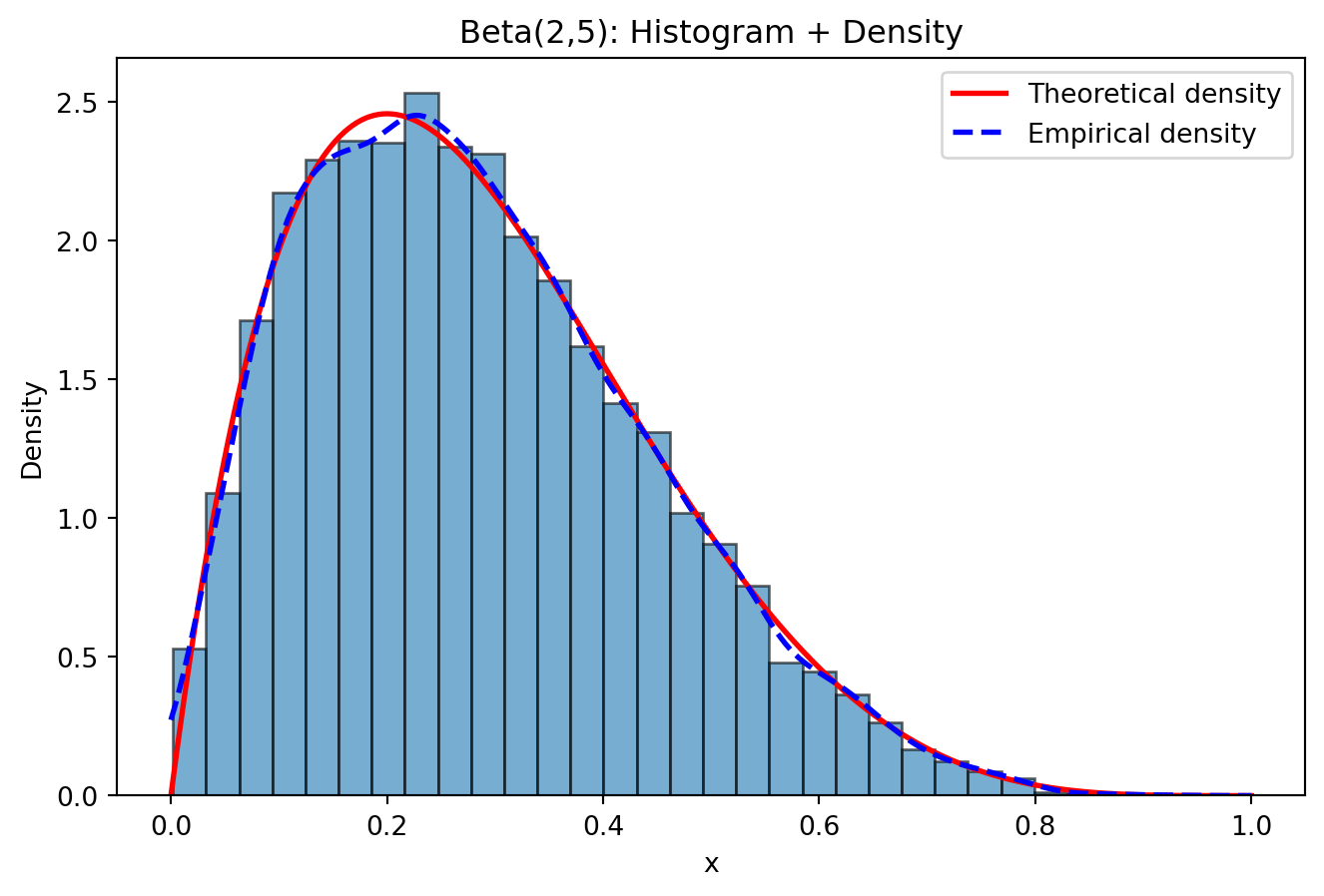
- Compute mean and variance.
emp_mean = np.mean(x)
emp_var  = np.var(x, ddof=1)

theo_mean = a / (a + b)
theo_var  = (a * b) / ((a + b)**2 * (a + b + 1))

print("Empirical mean:", emp_mean)
print("Theoretical mean:", theo_mean)
print("Empirical variance:", emp_var)
print("Theoretical variance:", theo_var)
Empirical mean: 0.28388702893411
Theoretical mean: 0.2857142857142857
Empirical variance: 0.025079505260659093
Theoretical variance: 0.025510204081632654- Repeat for:
- Beta(0.5, 0.5)
- Beta(5, 5)
def run_beta(a, b, n=10000, seed=123):
    np.random.seed(seed)
    x = beta.rvs(a, b, size=n)

    plt.figure(figsize=(8,5))
    plt.hist(x, bins=40, density=True, alpha=0.6, edgecolor='black',
             range=(0,1))

    xs = np.linspace(0, 1, 500)
    plt.plot(xs, beta.pdf(xs, a, b), 'r-', lw=2)

    plt.title(f"Beta({a}, {b})")
    plt.xlabel("x")
    plt.ylabel("Density")
    plt.show()

    emp_mean = np.mean(x)
    emp_var  = np.var(x, ddof=1)

    theo_mean = a / (a + b)
    theo_var  = (a * b) / ((a + b)**2 * (a + b + 1))

    print(f"\nBeta({a}, {b})")
    print("Empirical mean:", emp_mean, "  Theoretical mean:", theo_mean)
    print("Empirical var :", emp_var,  "  Theoretical var :", theo_var)

run_beta(2, 5)
run_beta(0.5, 0.5)
run_beta(5, 5)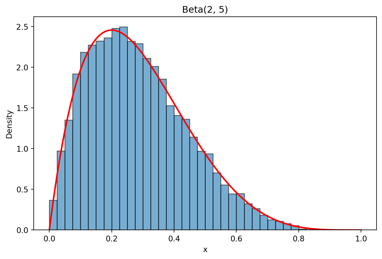
Beta(2, 5)
Empirical mean: 0.28388702893411   Theoretical mean: 0.2857142857142857
Empirical var : 0.025079505260659093   Theoretical var : 0.025510204081632654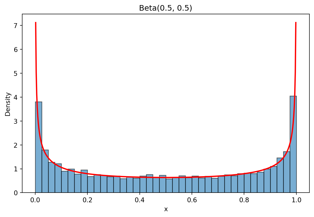
Beta(0.5, 0.5)
Empirical mean: 0.5023044733845982   Theoretical mean: 0.5
Empirical var : 0.1243420507711425   Theoretical var : 0.125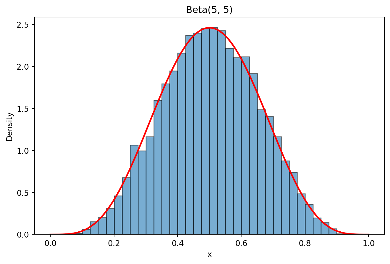
Beta(5, 5)
Empirical mean: 0.5018933069915179   Theoretical mean: 0.5
Empirical var : 0.022669247459073824 Theoretical var : 0.022727272727272728- How do the shape parameters affect:
- symmetry?
- concentration?
- boundary behaviour?
Symmetry
The Beta distribution is symmetric if and only if \(\alpha = \beta.\)
- If \(\alpha = \beta\) → symmetric around \(0.5\).
- If \(\alpha < \beta\) → distribution is skewed toward 0.
- If \(\alpha > \beta\) → distribution is skewed toward 1.
From 4):
- \(\text{Beta}(5,5)\) → symmetric and bell-shaped.
- \(\text{Beta}(2,5)\) → skewed toward 0.
- \(\text{Beta}(0.5,0.5)\) → symmetric but U-shaped.
Concentration (Spread Around the Mean)
The variance is:
\[ \mathrm{Var}(X) = \frac{\alpha \beta}{(\alpha + \beta)^2 (\alpha + \beta + 1)}. \]
As \(\alpha + \beta\) increases:
- The variance decreases.
- The distribution becomes more concentrated around the mean.
Thus:
- Large \(\alpha + \beta\) → tightly concentrated.
- Small \(\alpha + \beta\) → more spread out.
Boundary Behaviour (Near 0 and 1)
The density near the boundaries depends on whether parameters are less than 1.
Near 0:
- If \(\alpha < 1\) → density \(\to \infty\) at 0.
- If \(\alpha = 1\) → finite nonzero value at 0.
- If \(\alpha > 1\) → density \(\to 0\) at 0.
Near 1:
- If \(\beta < 1\) → density \(\to \infty\) at 1.
- If \(\beta = 1\) → finite nonzero value at 1.
- If \(\beta > 1\) → density \(\to 0\) at 1.
Examples:
- \(\text{Beta}(0.5,0.5)\) → spikes at both 0 and 1 (U-shaped).
- \(\text{Beta}(5,5)\) → zero at both boundaries, peak at 0.5.
- \(\text{Beta}(2,5)\) → zero at boundaries, skewed toward 0.
Exercise 4: Multinomial Distribution
Let
\[(X_1, X_2, X_3) \sim \text{Multinomial}(n=20, p=(0.2,0.5,0.3))\]
- Simulate 5,000 independent multinomial experiments.
- Compute:
- sample means of each component
- covariance matrix
- Verify: \(E[X_i] = np_i\)
- Verify that components are negatively correlated.
- Visualisation
- Scatterplot of \(X_1\) vs \(X_2\)
- Comment on dependence structure.
- Conceptual Question: Why must multinomial components be dependent?
Solution
- Simulate 5,000 independent multinomial experiments.
import numpy as np
import matplotlib.pyplot as plt
from scipy.stats import multinomial

np.random.seed(123)

B = 5000
n = 20
p = np.array([0.2, 0.5, 0.3])

# each row = one experiment, each column = X1, X2, X3
X = multinomial.rvs(n=n, p=p, size=B)- Compute:
- sample means of each component
- covariance matrix
# sample means of each component
sample_means = X.mean(axis=0)
print("Sample means:", sample_means)

# sample covariance matrix
sample_cov = np.cov(X, rowvar=False)
print("Sample covariance matrix:\n", sample_cov)
Sample means: [ 3.9878 10.03 5.9822]
Sample covariance matrix:
[[ 3.1266765 -1.94962392 -1.17705257]
[-1.94962392 4.93968794 -2.99006401]
[-1.17705257 -2.99006401 4.16711658]]By LLN, sample means (empirical averages) are close to:
\[ E[X_i] = np_i \]
- \(20 \times 0.2 = 4,\)
- \(20 \times 0.5 = 10,\)
- \(20 \times 0.3 = 6,\)
and the covariance matrix is in the form of:
\[ \begin{pmatrix} \mathrm{Var}(X_1) & \mathrm{Cov}(X_1,X_2) & \mathrm{Cov}(X_1,X_3) \\ \mathrm{Cov}(X_2,X_1) & \mathrm{Var}(X_2) & \mathrm{Cov}(X_2,X_3) \\ \mathrm{Cov}(X_3,X_1) & \mathrm{Cov}(X_3,X_2) & \mathrm{Var}(X_3) \end{pmatrix} \]
- In theory, \(Var(X_i)=np_i(1-p_i) > 0\).
- For covariance, \(Cov(X_i, X_j) = -np_ip_j \quad(i\neq j)\).
- Covariances are negative because an increase in \(X_i\) must result in a decrease in \(X_j, (i\neq j)\).
- Since the variables move in opposite directions, we have negative covariance.
- Verify: \(E[X_i] = np_i\)
theo_means = n * p
np.column_stack((sample_means, theo_means))
array([[ 3.9878, 4. ],
[10.03 , 10. ],
[ 5.9822, 6. ]])- Verify that components are negatively correlated.
sample_cor = np.corrcoef(X, rowvar=False)
print("Sample correlation matrix:\n", sample_cor)
Sample correlation matrix:
[[ 1. -0.49608902 -0.32608931]
[-0.49608902 1. -0.65904171]
[-0.32608931 -0.65904171 1. ]]Note that:
\[ \mathrm{Corr}(X_i, X_i)=\frac{\mathrm{Cov}(X_i, X_i)} {\sqrt{\mathrm{Var}(X_i)\mathrm{Var}(X_i)}} \]
- The covariance matrix measures joint variability in original units, while the correlation matrix standardises this to measure pure strength of linear dependence on a -1 to 1 scale.
- In a correlation matrix, the diagonal entries are always 1, because a variable is perfectly positively linearly related to itself.
- Visualisation
- Scatterplot of \(X_1\) vs \(X_2\)
- Comment on dependence structure.
plt.figure(figsize=(6,5))
plt.scatter(X[:,0], X[:,1], alpha=0.5, s=12)
plt.xlabel("X1")
plt.ylabel("X2")
plt.title("Scatterplot of X1 vs X2 (Multinomial, n=20)")
plt.show()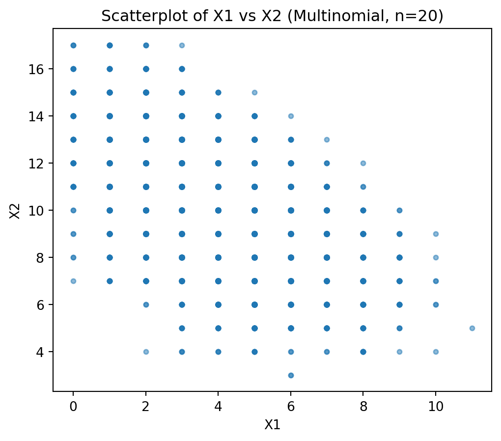
You should see a downward trend. When \(X_1\) is large, \(X_2\) tends to be smaller (and vice versa).
Also, the points lie within feasible integer bounds, especially because:
\[ X_1+X_2+X_3=20. \]
So not every pair \((X_1,X_2)\) is possible; they’re constrained by the remaining count for \(X_3\).
- Conceptual Question: Why must multinomial components be dependent?
Because the components must sum to a fixed total:
\[ X_1+X_2+X_3=n. \]
So if one component increases, at least one of the others must decrease to keep the sum equal to \(n\). This fixed-sum constraint forces dependence and typically creates negative correlations between different categories.
10.1 Part 2: Joint distributions and dependence
Exercise 5
Explain why dependence matters in simulation. Give 3 examples.
Dependence in simulation means that variables or events influence each other rather than occurring independently. If dependence is ignored, simulations can produce unrealistic results because many real-world processes are correlated.
Why it matters: Modeling dependence helps simulations reflect real system behavior, improving accuracy and decision-making.
Examples:
- Finance: Stock returns often move together (correlation between assets). Ignoring this can underestimate portfolio risk.
- Healthcare: A patient’s future health outcomes depend on their current condition and previous treatments.
- Traffic simulation: Congestion on one road affects traffic flow on nearby roads.
Exercise 6: Visualising Dependence
Simulate two scenarios:
Case A: Independent variables
Let: \[ X \sim \mathcal{N}(0,1), \quad Y \sim \mathcal{N}(0,1) \]
Generate independently.
Case B: Dependent variables
Define:
\[ Y = 0.8X + \sqrt{1-0.8^2} Z \]
where \(Z \sim \mathcal{N}(0,1)\) independent of \(X\).
- Generate 5,000 observations for each case.
- Produce scatterplots.
- Compute correlation.
- Compare visually and numerically.
import numpy as np
from scipy.stats import pearsonr
import matplotlib.pyplot as plt

# Case A: Independent
np.random.seed(123)
x = np.random.normal(size=5000)
y = np.random.normal(size=5000)

# Case B: Dependent
z = np.random.normal(size=5000)
y2 = 0.8*x + np.sqrt(1 - 0.8**2) * z

# Plots
plt.figure(figsize=(10,4))

plt.subplot(1,2,1)
plt.scatter(x, y, s=5)
plt.title("Case A: Independent")

plt.subplot(1,2,2)
plt.scatter(x, y2, s=5)
plt.title("Case B: Dependent")

plt.tight_layout()
plt.show()

# Correlations
print("Case A correlation:", round(pearsonr(x, y)[0], 3))
print("Case B correlation:", round(pearsonr(x, y2)[0], 3))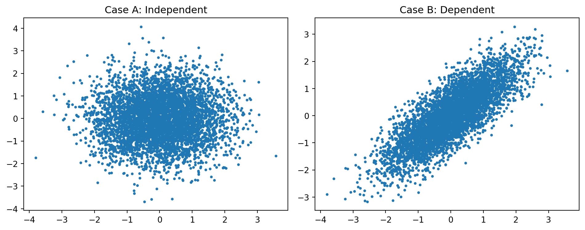
Case A correlation: 0.002
Case B correlation: 0.799
Comments:
Case A’s scatterplot should look like random circular cloud with no directional trend (\(\rho \approx 0\)).
Case B’s scatterplot should show clear upward diagonal, elongate ellipse (\(\rho \approx 0.8\)).
This construction is important because it is exactly how multivariate normal simulation works. In fact, the general idea is \[ Y = \rho X + \sqrt{1-\rho^2}\,Z \]
which produces correation \(\rho\)
Exercise 7: Constructing a Joint Distribution (Discrete)
Let:
\[ P(X=0,Y=0)=0.2, \quad P(X=0,Y=1)=0.3, \] \[ P(X=1,Y=0)=0.1, \quad P(X=1,Y=1)=0.4 \]
- Verify probabilities sum to 1.
Check that
\[ \sum_x \sum_y p_{X,Y}(x,y) = 1. \]
0.2+0.3+0.1+0.41.0- Compute marginal distributions.
- For \(x=0\), \(P(X=0) = 0.2 + 0.3 = 0.5.\)
- For \(x=1\), \(P(X=1) = 0.1 + 0.4 = 0.5.\)
\[ \therefore p_X(x) = \begin{cases} 0.5, & x=0,1 \\ 0, & \text{otherwise.} \end{cases} \]
- For \(y=0\), \(P(Y=0) = 0.2 + 0.1 = 0.3.\)
- For \(y=1\), \(P(Y=1) = 0.3 + 0.4 = 0.7.\)
\[ \therefore p_Y(y) = \begin{cases} 0.3, & y=0 \\ 0.7, & y=1 \\ 0, \text{otherwise.} \end{cases} \]
- Check if independent.
\[ p(x,y) = p_X(x) \, p_Y(y) \]
| \(X\) | \(Y\) | \(P(X,Y)\) |
|---|---|---|
| 0 | 0 | 0.2 |
| 0 | 1 | 0.3 |
| 1 | 0 | 0.1 |
| 1 | 1 | 0.4 |
For the \((X=0, Y=0)\) case,
\[ p_X(x) \, p_Y(y) = 0.5 \times 0.3 = 0.15. \]
However, \(P(X=0, Y=0) = 0.2 \neq 0.15.\) The independence condition fails.
- Compute covariance manually.
\[ \text{Cov}(X,Y) = E(XY) - E(X)E(Y) \]
Calculate \(E(X)\), \(E(Y)\) and \(E(XY)\)
\[ E(X) = \sum x P(X=x) = 0(0.5) + 1(0.5) = 0.5 \]
\[ E(Y) = \sum y P(Y=y) = 0(0.3) + 1(0.7) = 0.7 \]
| \(X\) | \(Y\) | \(P(X,Y)\) | \(XY\) | \(XY\times P\) |
|---|---|---|---|---|
| 0 | 0 | 0.2 | 0 | 0 |
| 0 | 1 | 0.3 | 0 | 0 |
| 1 | 0 | 0.1 | 0 | 0 |
| 1 | 1 | 0.4 | 1 | 0.4 |
\[ E(XY) = 0.4 \]
\[ \text{Cov}(X,Y) = 0.4 - 0.5(0.7) = 0.4 - 0.35 = 0.05 \]
- Simulate 10,000 draws from this joint distribution.
import numpy as np
import pandas as pd

np.random.seed(123)
n = 10000

# Support values
X = np.array([0, 0, 1, 1])
Y = np.array([0, 1, 0, 1])

# Probabilities
p = np.array([0.2, 0.3, 0.1, 0.4])

# Sample indices 0–3 (Python is 0‑based)
s = np.random.choice(4, size=n, replace=True, p=p)

# Simulated values
X_sim = X[s]
Y_sim = Y[s]

# Joint empirical distribution (like table(X_sim, Y_sim)/n)
joint = pd.crosstab(X_sim, Y_sim, normalize=True)

print(joint)
col_0 0 1
row_0
0 0.2064 0.2901
1 0.1020 0.4015- Compare empirical and theoretical covariance.
np.cov(X_sim, Y_sim, bias=True)[0, 1]np.float64(0.053279400000000025)Comments:
From Question 4, the theoretical covariance is 0.05. The simulated covariance should be close to 0.05, with small differences due to random sampling variation. As the sample size increases, the empirical covariance tends to approach the theoretical covariance.
Exercise 8: Zero Correlation ≠ Independence
Let:
\[ X \sim \mathcal{N}(0,1) \]
Define:
\[ Y = X^2 \]
- Simulate 10,000 observations.
- Compute correlation.
- Plot scatterplot.
- Explain why they are dependent despite near-zero correlation.
np.random.seed(123)

# Data
x = np.random.normal(size=10000)
y = x**2

# Correlation
print("Correlation:", pearsonr(x, y)[0])

# Plot
plt.scatter(x, y, s=5)
plt.title("Scatterplot of Y = X^2")
plt.xlabel("X")
plt.ylabel("Y")
plt.show()
Correlation: 0.01710437679261658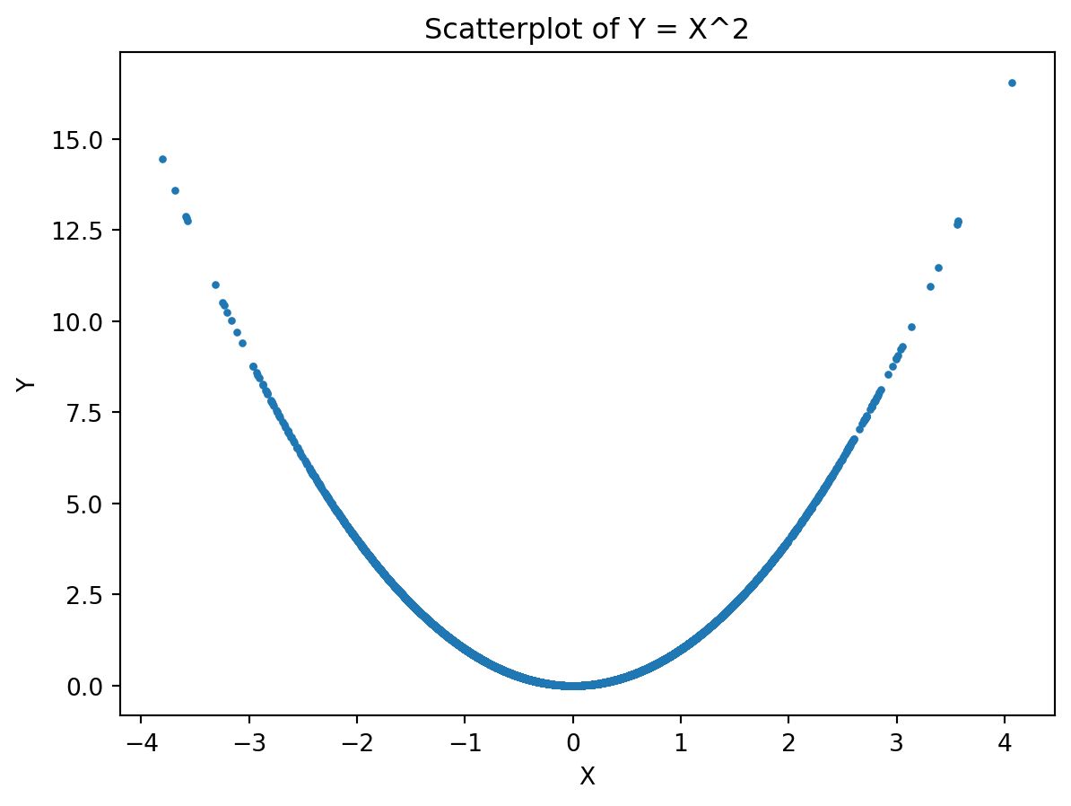
Comments:
The scatterplot should show a U-shaped parabola, because every point lies on \(Y=X^2\). So the relationship is clearly deterministic and nonlinear.
The sample correlation should be close to 0, though not exactly 0 in finite samples.
Although the correlation between \(X\) and \(Y\) is close to 0, \(X\) and \(Y\) are not independent because \(Y\) is completely determined by \(X\) through the relationship \(Y=X^2\). Knowing the value of \(X\) tells us the exact value of \(Y\), so there is clear dependence. The correlation is near zero only because correlation measures linear association, whereas the relationship here is nonlinear and symmetric around 0.
Zero correlation means no linear relationship, not no relationship at all.
Why is the correlation near zero?
Correlation measures linear association. Here,
\[ \operatorname{Corr}(X,Y)=\operatorname{Corr}(X,X^2). \]
Since \(X \sim \mathcal N(0,1)\),
\[ \operatorname{Cov}(X,X^2)=E(X^3)-E(X)E(X^2). \]
Now:
- \(E(X)=0\)
- \(E(X^2)=1\)
- \(E(X^3)=0\) because the normal distribution is symmetric about 0
So
\[ \operatorname{Cov}(X,X^2)=0-0\cdot 1=0. \]
Hence,
\[ \operatorname{Corr}(X,X^2)=0. \]
So the near-zero sample correlation is exactly what theory predicts.
Exercise 9: Conditional Simulation
Let:
\[ X \sim \text{Gamma}(2,1) \]
Given \(X=x,\)
\[ Y|X=x \sim \text{Poisson}(x) \]
- Simulate 5,000 pairs.
- Plot scatterplot.
- Estimate:
- \(E[Y]\)
- Compare with theoretical value using law of total expectation.
# Seed
np.random.seed(123)

# Sample size
n = 5000

# X ~ Gamma(shape=2, rate=1)  --> in scipy: scale = 1/rate = 1
x = np.random.gamma(shape=2, scale=1, size=n)

# Y | X ~ Poisson(X)
y = np.random.poisson(lam=x)

# Plot
plt.scatter(x, y, s=5)
plt.xlabel("X")
plt.ylabel("Y")
plt.title("Conditional simulation: Y | X ~ Poisson(X)")
plt.show()

# Mean of Y
print(np.mean(y))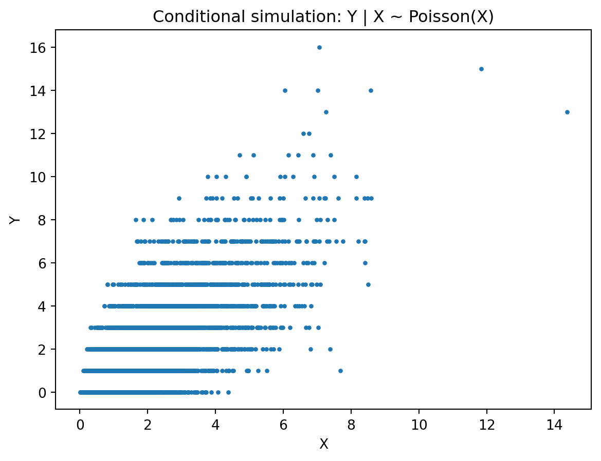
2.0386Theoretical Value Using The Law of Total Expectation
\[ E[Y] = E[E(Y|X)] = \int E[Y \mid X=x]\,f_X(x)\,dx \]
Since
\[ Y \mid X = x \sim \text{Poisson}(x), \]
the conditional mean is
\[ E[Y \mid X=x] = x. \]
So
\[ E[Y] = E[E(Y \mid X)] = E[X]. \]
Now if
\[ X \sim \text{Gamma}(2,1), \]
with shape 2 and rate 1, then
\[ E[X] = 2/1 = 2. \]
Therefore,
\[ E[Y] = 2. \]
Exercise 10: Simulating Bivariate Normal
Construct a portfolio simulation:
Let:
- \(X_1, X_2\) be correlated returns (bivariate normal).
- Portfolio return:
\[ R = 0.6X_1 + 0.4X_2 \]
Tasks:
- Simulate 10,000 returns.
- Estimate variance.
- Plot scatterplot and explain.
- Explain how ignoring dependence affects risk estimation.
We can simulate correlated normals using a linear transformation:
\[ X_1 = Z_1, \quad X_2 = \rho Z_1 + \sqrt{1-\rho^2} \, Z_2. \]
np.random.seed(123)

n = 10000
rho = 0.7

# Two independent standard normals
z1 = np.random.normal(size=n)
z2 = np.random.normal(size=n)

# Linear transformation
x1 = z1
x2 = rho * z1 + np.sqrt(1 - rho**2) * z2

# Portfolio return
R = 0.6 * x1 + 0.4 * x2

# Estimate portfolio variance
print(np.var(R, ddof=1)) # ddof=1 matches R's var() which divides by n-10.8563345297342178Extra: We can also compare this with the theoretical variance.
Since
\[ R = 0.6 X_1 + 0.4 X_2, \]
the variance is
\[ \text{Var}(R) = 0.6^2 \text{Var}(X_1) + 0.4^2 \text{Var}(X_2) + 2(0.6)(0.4)\text{Cov}(X_1,X_2). \]
Because \(\text{Var}(X_1) = \text{Var}(X_2) = 1\) and \(\text{Cov}(X_1,X_2) = \rho = 0.7,\)
we get
\[ \text{Var}(R) = 0.36 + 0.16 + 2(0.6)(0.4)(0.7) = 0.856 \]
So the simulated variance should be close to 0.856.
plt.scatter(x1, x2, s=5)
plt.xlabel(r"$X_1$")
plt.ylabel(r"$X_2$")
plt.title("Scatterplot of correlated returns")
plt.show()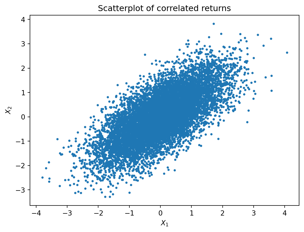
Comments:
The scatterplot should show an upward-sloping cloud of points. This indicates positive dependence: when \(X_1\) is high, \(X_2\) also tends to be high; when \(X_1\) is low, \(X_2\) tends to be low. Because the variables are jointly normal, the cloud has an elliptical shape. This matters for the portfolio because the two asset returns do not move independently. Their co-movement contributes directly to the total portfolio variance.
# Variance if independence were incorrectly assumed
0.6**2 + 0.4**20.52Comments:
If we incorrectly assume independence, then we set
\[ \text{Cov}(X_1, X_2) = 0. \]
The portfolio variance would then be estimated as
\[ \text{Var}(R) = 0.6^2(1) + 0.4^2(1) = 0.52. \]
But the correct variance is 0.856. So ignoring the positive dependence would underestimate risk.
When returns are positively correlated, the two assets tend to rise and fall together. This reduces diversification benefits, so the portfolio is riskier than it would be under independence.
More generally:
- positive dependence → higher portfolio risk than independence suggests
- negative dependence → lower portfolio risk and stronger diversification benefits
So modelling dependence correctly is essential in portfolio simulation.
Exercise 11
(Jones et al., 2014, Chapter 14, Exercise 23, p. 282)
A diagnostic test is used to determine whether or not a person has a certain disease. If the test is positive, then it is assumed the person has the disease; if negative, that they do not have it. However, the test is not 100% accurate.
- If a diseased person is tested, it gives a negative result 5% of the time (a false negative).
- When testing a person free of the disease, it gives a false positive 10% of the time.
- Suppose we choose someone at random from a population in which only 1 person in 50 has the disease.
- Find the probability that their test result is positive.
- Find the probability that their test result is misleading.
- Find the probability that they actually have the disease if they test positive.
Define events:
- \(D\): person has the disease
- \(D^c\): person does not have the disease
- \(+\): positive test
- \(-\): negative test
From the problem:
\[ P(D) = \frac{1}{50} = 0.02, \qquad P(D^c) = 0.98 \]
False negative rate:
\[ P(-|D) = 0.05 \]
Therefore
\[ P(+|D) = 1 - 0.05 = 0.95 \]
False positive rate:
\[ P(+|D^c) = 0.10 \]
Thus
\[ P(-|D^c) = 0.90 \]
- Probability the test result is positive
Using the law of total probability,
\[ P(+) = P(+|D)P(D) + P(+|D^c)P(D^c) \]
Substituting the values:
\[ P(+) = 0.95(0.02) + 0.10(0.98) \]
\[ P(+) = 0.019 + 0.098 = 0.117 \]
Therefore,
\[ \boxed{P(+) = 0.117} \]
About 11.7% of tests are positive.
- Probability the test result is misleading
A misleading result occurs if the test gives:
- a false positive (test positive but no disease), or
- a false negative (test negative but disease present).
Thus
\[ P(\text{misleading}) = P(+|D^c)P(D^c) + P(-|D)P(D) \]
Compute each term:
False positive probability:
\[ 0.10 \times 0.98 = 0.098 \]
False negative probability:
\[ 0.05 \times 0.02 = 0.001 \]
Total probability:
\[ P(\text{misleading}) = 0.098 + 0.001 = 0.099 \]
Hence,
\[ \boxed{P(\text{misleading}) = 0.099} \]
So approximately 9.9% of test results are incorrect.
- Probability the person has the disease given a positive test
Using Bayes’ theorem,
\[ P(D|+) = \frac{P(+|D)P(D)}{P(+)} \]
Substitute values:
\[ P(D|+) = \frac{0.95(0.02)}{0.117} \]
\[ P(D|+) = \frac{0.019}{0.117} \]
\[ P(D|+) \approx 0.162 \]
Therefore,
\[ \boxed{P(D|+) \approx 0.162} \]
Note
Even though the test has high accuracy (95% sensitivity and 90% specificity), the disease is rare (only 2% prevalence). As a result, many positive tests are false positives. Only about 16% of people who test positive actually have the disease.
Exercise 12
(Jones et al., 2014, Chapter 14, Exercise 24, p. 282)
There are two bus lines which travel between towns \(A\) and \(B\).
Bus line \(A\) runs late 20% of the time, while bus line \(B\) runs late 50% of the time. You travel three times as often by line \(A\) as you do by line \(B\). On a certain day you arrive late. What is the probability that you used bus line \(B\) that day?
Let
- \(A\): you took bus line A
- \(B\): you took bus line B
- \(L\): the bus arrives late
You travel three times as often on line \(A\) as on line \(B\), so the ratio is
\[ P(A):P(B) = 3:1 \]
Thus
\[ P(A) = \frac{3}{4}, \qquad P(B) = \frac{1}{4}. \]
From the problem:
\[ P(L|A) = 0.20, \quad P(L|B) = 0.50 \]
Using the law of total probability
\[ P(L) = P(L|A)P(A) + P(L|B)P(B) \]
Substitute the values:
\[ \begin{aligned} P(L) &= 0.20\left(\frac{3}{4}\right) + 0.50\left(\frac{1}{4}\right) \\ &= 0.15 + 0.125 = 0.275 \end{aligned} \]
We want the probability that you took bus line \(B\) given that you arrived late. Using Bayes’ theorem
\[ \begin{aligned} P(B|L) &= \frac{P(L|B)P(B)}{P(L)} \\ &=\frac{0.50 \times 0.25}{0.275} \\ &=\frac{0.125}{0.275} \end{aligned} \]
\[ \boxed{P(B|L) \approx 0.455} \]
Note
Even though bus line \(A\) is used more often, bus line \(B\) is much more likely to run late. Observing a late arrival increases the probability that bus \(B\) was used.
Exercise 13
(Jones et al., 2014, Chapter 14, Exercise 26, p. 283)
The dice game craps is played as follows. The player throws two dice, and if the sum is seven or eleven, then he wins. If the sum is two, three, or twelve, then he loses. If the sum is anything else, then he continues throwing until he either throws that number again (in which case he wins) or he throws a seven (in which case he loses). Calculate the probability that the player wins.
In the dice game craps, a player throws two dice.
- If the sum is 7 or 11, the player wins immediately.
- If the sum is 2, 3, or 12, the player loses immediately.
- Otherwise, the sum becomes the point. The player keeps rolling until:
- the point appears again (win), or
- a 7 appears (loss).
Two dice have 36 equally likely outcomes. The following table shows the sum of die 1 and die 2, where rows are value of die 1 and columns are value of die 2.
\[ \begin{array}{c|cccccc} & 1 & 2 & 3 & 4 & 5 & 6 \\ \hline 1 & \textbf{\color{red}2} & \textbf{\color{red}3} & 4 & 5 & 6 & \textbf{\color{green}7} \\ 2 & \textbf{\color{red}3} & 4 & 5 & 6 & \textbf{\color{green}7} & 8 \\ 3 & 4 & 5 & 6 & \textbf{\color{green}7} & 8 & 9 \\ 4 & 5 & 6 & \textbf{\color{green}7} & 8 & 9 & 10 \\ 5 & 6 & \textbf{\color{green}7} & 8 & 9 & 10 & \textbf{\color{green}11} \\ 6 & \textbf{\color{green}7} & 8 & 9 & 10 & \textbf{\color{green}11} & \textbf{\color{red}12} \end{array} \]
Immediate win:
The order matters when counting outcomes for two dice. When rolling two dice, the outcomes are ordered pairs \((d_1,d_2)\). Thus, the two immediate win events are
\[ \begin{aligned} \text{Sum } &= 7: \{(1,6),(2,5),(3,4),(4,3),(5,2),(6,1)\} \\ \text{Sum } &= 11: \{(5,6),(6,5)\} \end{aligned} \]
\[ P(\text{win immediately}) = \frac{6}{36} + \frac{2}{36} = \frac{8}{36} \]
Immediate loss:
\[ P(\text{lose immediately}) = \frac{1}{36} + \frac{2}{36} + \frac{1}{36} = \frac{4}{36} \]
Possible points are
\[ 4,5,6,8,9,10 \]
Probabilities of establising each point from the first roll of the dice are
\[ \begin{array}{ccc} \text{Sum } (k) & \text{Ways} & P(k)\\ \hline 4 & 3 & 3/36 \\ 5 & 4 & 4/36\\ 6 & 5 & 5/36\\ 8 & 5 & 5/36\\ 9 & 4 & 4/36\\ 10 & 3 & 3/36\\ \end{array} \]
If the point is \(k\), the player wins if \(k\) appears before a 7. Thus
\[ P(\text{win} \mid k) = \frac{P(k)}{P(k)+P(7)}. \]
Since \(P(7)=6/36\),
\[ P(\text{win} \mid k)= \begin{cases} \dfrac{3/36}{3/36 + 6/36}=\dfrac13, & k = 4,10, \\[1em] \dfrac{4/36}{4/36 + 6/36}=\dfrac25, & k = 5,9, \\[1em] \dfrac{5/36}{5/36 + 6/36}=\dfrac{5}{11}, & k = 6,8. \end{cases} \]
\[ \begin{aligned} P(\text{win}) &= P(\text{win immediately}) + \sum_k P(k)\,P(\text{win}\mid k) \\ &= \frac{8}{36} + 2\left(\frac{3}{36}\cdot\frac13\right) + 2\left(\frac{4}{36}\cdot\frac25\right) + 2\left(\frac{5}{36}\cdot\frac{5}{11}\right) \\ &= \frac{8}{36}+\frac{2}{36}+\frac{4}{45}+\frac{25}{198}. \end{aligned} \]
\[ \boxed{P(\text{win}) \approx 0.493} \]
The player wins about 49.3% of the time, giving the casino a small advantage.
Extra Exercises
Distribution Identification
For each of the functions below check if it is a valid cumulative distribution function (cdf), probability density function (pdf) or a probability mass function (pmf). For valid cdf’s, compute the corresponding pdf or pmf. Also for each valid pdf or pmf compute the corresponding cdf.
\[ f_X(x) = \begin{cases} 6x - 6x^2 & 0 \le x \le 1 \\ 0 & \text{Otherwise} \end{cases} \]
Check:
\[ f_X(x) \geq 0, \qquad 0\leq x \leq 1 \]
and
\[ \int_0^1 f_X(x)\,dx = \int_0^1 6x-6x^2 =1, \]
it is a valid pdf.
\[ F_X(x) = \begin{cases} 0 & x < 0 \\ 0.2 & 0 < x \le 1 \\ 0.3 & 1 < x \le 2 \\ 1 & x > 2 \end{cases} \]
Properties of a CDF
A function \(F_X(x)\) is a valid CDF if it satisfies:
- Non-decreasing
\[ F(x_1) \le F(x_2) \quad \text{for } x_1 < x_2 \]
- Right-continuity
\[ F(x) = \lim_{t \downarrow x} F(t) \]
- Limits
\[ \lim_{x\to -\infty} F(x) = 0, \qquad \lim_{x\to \infty} F(x) = 1 \]
However, in the given function \(F(0)\) is not defined.
Also, at \(x=1\):
\[ F(1)=0.2 \]
but
\[ \lim_{x\downarrow1}F(x)=0.3 \]
Thus
\[ F(1) \neq \lim_{x\downarrow1}F(x) \]
so the function is not right-continuous.
The function is not a valid CDF because it is not defined at some points and it is not right-continuous.
Scenario Analysis
For each of the scenarios below identify
- Random Variable
- Distribution and paramenters
- Probability (mass) density function
- Probability of interest
You may use direct calculations, use R or any other computing system.
- A husband has 6 tasks on his to-do list and a wife has 10 tasks on her to-do list. Four tasks are randomly picked up. We are interested in the number of tasks the wife will have to do. What is the probability that wife would have to do all four tasks.
\[ X = \text{number of tasks the wife will do} \]
\[ X \sim \text{Hypergeometric}(N=16,\; M=10,\; n=4) \]
\[ P(X=4) = \frac{\binom{10}{4}\binom{6}{0}}{\binom{16}{4}} = 0.11538 \]
import scipy.stats as ss
M = 10      # number of white balls
N = 16      # total balls (10 white + 6 black)
n = 4       # draws
x = 4       # observed white balls
print(round(ss.hypergeom.pmf(x, N, M, n), 4))0.1154- A couple likes to play chess together. Male is not good at the game and has only 10% chance of winning. The stubborn couple decides to play until male wins two games. We are interested in number of games couple would have to play. What is the probability that couple would play at least 15 games?
\[ X = \text{number of games until the second win by a male} \]
\[ X \sim \text{Negative Binomial}(r = 2,\; p = 0.1) \]
\[ P(X \ge 15) = 0.5846 \]
size = 2        # number of successes
prob = 0.1      # success probability
print(round(ss.nbinom.sf(12, size, prob), 4)) # sf = 1 - cdf0.5846- A student is taking a true/false test that consists of 10 questions. The student has approximately 80% change of getting any individual question correct. We are interested in the number of questions a student answers correctly. What is the probability that student gets all ten questions right?
\[ X = \text{number of questions a student answers correctly out of 10} \]
\[ X \sim \text{Binomial}(n = 10,\; p = 0.8) \]
\[ P(X = 10) = 0.10737 \]
print(round(ss.binom.pmf(10, n=10, p=0.8), 4))0.1074- A police officer has found that approximately 0.1% of the vehicles he pulls over fail the alcohol test. He is interested in the number of vehicles that will fail the alcohol test from next 100 vehicles he pulls over. What this the probability that 5 vehicles will fail the alcohol test from next 100 vehicles he pulls over?
\[ X = \text{number of vehicles that will fail the alcohol test out of the next 100} \]
\[ X \sim \text{Poisson}(\lambda = 0.1) \]
\[ P(X = 5) = 0 \]
print(round(ss.poisson.pmf(5, mu=0.1), 4))0.0- At a certain manufacturing company, approximately 2% of the products are defective. We are interested in the number of products that need to be checked before we hit rst defective item. What is the probability that third product checked will be rst defective item?
\[ X = \text{number of products checked to get a defective} \]
\[ X \sim \text{Geometric}(p = 0.02) \]
\[ P(X = 3) = 0.01921 \]
print(round(ss.geom.pmf(2, p=0.02), 4))0.0196- The amount of time one spends in a bank is exponentially distributed with mean 10 minutes. What is the probability that the customer will spend more than 15 minutes in the bank?
\[ X = \text{time spent in a bank} \]
\[ X \sim \text{Exponential}(\lambda = 0.1) \]
\[ P(X > 15) = \int_{15}^{\infty} 0.1 e^{-0.1x}\, dx = e^{-0.1 \times 15} \]
print(round(ss.expon.sf(15, scale=1/0.1), 4)) # scale = 1/lambda0.2231- The smiling times of babies, in seconds, follow a uniform distribution between 0 and 23 seconds, inclusive. What is the probability that a randomly selected eight week old baby smiles between 2 and 18 seconds?
\[ X = \text{smiling times} \]
\[ X \sim \text{Uniform}(0, 23) \]
\[ P(2 < X < 18) = \int_{2}^{18} \frac{1}{23}\, dx = 0.6957 \]
print(round((ss.uniform.cdf(18, loc=0, scale=23) - ss.uniform.cdf(2, loc=0, scale=23)), 4))0.6957- A utility industry consultant predicts a cutback in the utility industry by a percentage speci ed by a Beta distribution with parameters \(\alpha = 1\) and \(\beta = 0.25\), in ve year period. What is the probability that Department of Hydrology will down size by 10% to 30%?
\[ X = \text{cutback in utility industry (\%)} \]
\[ X \sim \text{Beta}(1,\; 0.25) \]
\[ f_X(x) = \frac{x^{1-1}(1-x)^{0.25-1}}{B(1, 0.25)} \]
\[ B(1, 0.25) = \frac{\Gamma(1)\,\Gamma(0.25)}{\Gamma(1.25)} = \frac{1}{0.25} \]
\[ \int_{0.1}^{0.3} f_X(x)\, dx = \int_{0.1}^{0.3} \frac{x^{1-1}(1-x)^{0.25-1}}{B(1, 0.25)}\, dx = 0.0593 \]
print(round(ss.beta.cdf(0.3, a=1, b=0.25) - ss.beta.cdf(0.1, a=1, b=0.25), 4))0.0593Joint Distributions and Dependence
- Let \((X_1, X_2)\) and \((Y_1, Y_2)\) be two discrete random vectors with the following probability functions:
Joint pmf of \((X_1, X_2)\):
\[ \begin{array}{c|cc} f_{(X_1, X_2)}(x_1,x_2) & -1 & 1 \\ \hline 0 & 1/6 & 1/6 \\ 1/2 & 1/3 & 1/3 \end{array} \]
Joint pmf of \((Y_1, Y_2)\):
\[ \begin{array}{c|cc} f_{(Y_1, Y_2)}(y_1,y_2) & -1 & 1 \\ \hline 0 & 1/3 & 0 \\ 1 & 1/6 & 1/4 \\ 2 & 0 & 1/4 \end{array} \]
Show that \(X_2\) and \(Y_2\) are identically distributed.
\[ P[X_2 = x_2] = \begin{cases} -1, & 1/6 + 1/3 = 1/2, \\[6pt] 1, & 1/6 + 1/3 = 1/2. \end{cases} \]
\[ P[Y_2 = y_2] = \begin{cases} -1, & 1/3 + 1/6 + 0 = 1/2, \\[6pt] 1, & 0 + 1/4 + 1/4 = 1/2. \end{cases} \]
As \(X_2\) and \(Y_2\) take identical values with equal probability, they are identically distributed.
- Let \(X \sim N(7, 3^2)\), \(Y \sim N(5, 2^2)\) and \(\mathrm{Cor}(X,Y) = -0.2\).
- Specify the joint probability density function for \((X,Y)\).
\[ f_{X,Y}(x,y) = \frac{1}{2\pi \cdot 3 \cdot 2 \sqrt{1 - (-0.2)^2}} \exp\!\left(\frac{-z}{2\left(1 - (-0.2)^2\right)}\right) \]
where \(z\) is
\[ z = \frac{(x - 7)^2}{3^2} + \frac{(y - 5)^2}{2^2} - \frac{2(-0.2)(x - 7)(y - 5)}{3 \cdot 2}. \]
- Find the distribution for \(Z = 3X + 4Y\), hence find \(P[Z > 50]\).
Since \((X,Y)\) is jointly normal, any linear combination is also normal.
Thus \(Z\) is normally distributed with
\[ E[Z] = 3E[X] + 4E[Y] = 3(7) + 4(5) = 41. \]
The variance is
\[ \operatorname{Var}(Z) = 3^2 \operatorname{Var}(X) + 4^2 \operatorname{Var}(Y) + 2(3)(4)\operatorname{Cov}(X,Y). \]
Because
\[ \operatorname{Cov}(X,Y) = \rho \sigma_X \sigma_Y = (-0.2)(3)(2) = -1.2, \]
we obtain
\[ \operatorname{Var}(Z) = 9(9) + 16(4) + 2(3)(4)(-1.2) = 81 + 64 - 28.8 = 116.2. \]
Therefore
\[ Z \sim N(41,\; 116.2), \qquad \sigma_Z = \sqrt{116.2}. \]
To compute the probability:
\[ P(Z > 50) = 1 - \Phi\!\left( \frac{50 - 41}{\sqrt{116.2}} \right) = 1 - \Phi(0.835). \]
muZ = 3*7 + 4*5
varZ = 3**2 * 3**2 + 4**2 * 2**2 + 2*3*4*(-0.2*3*2)
sdZ = np.sqrt(varZ)
print(round((1 - ss.norm.cdf(50, loc=muZ, scale=sdZ)), 4))0.2019- Find the distribution for \(Z = X - Y\), hence find \(P[Z < 0]\).
Since \((X,Y)\) is jointly normal, any linear combination is also normal.
Thus \(Z\) is normally distributed with
\[ E[Z] = E[X] - E[Y] = 7 - 5 = 2. \]
The variance is
\[ \operatorname{Var}(Z) = \operatorname{Var}(X) + \operatorname{Var}(Y) - 2\,\operatorname{Cov}(X,Y). \]
Because
\[ \operatorname{Cov}(X,Y) = \rho \sigma_X \sigma_Y = (-0.2)(3)(2) = -1.2, \]
we obtain
\[ \operatorname{Var}(Z) = 9 + 4 - 2(-1.2) = 13 + 2.4 = 15.4. \]
Therefore
\[ Z \sim N(2,\; 15.4), \qquad \sigma_Z = \sqrt{15.4}. \]
To compute the probability:
\[ P(Z < 0) = \Phi\!\left( \frac{0 - 2}{\sqrt{15.4}} \right) = \Phi(-0.509). \]
muZ = 7 - 5
varZ = 3**2 + 2**2 - 2 * (-0.2 * 3 * 2)
sdZ = np.sqrt(varZ)

print(round(ss.norm.cdf(0, loc=muZ, scale=sdZ), 4))0.3051- Specify the distribution of \(Z = 3 + 4X + 2Y\).
Since \((X,Y)\) is jointly normal, any linear combination is also normal.
Thus \(Z\) is normally distributed with
\[ E[Z] = 3 + 4E[X] + 2E[Y] = 3 + 4(7) + 2(5) = 3 + 28 + 10 = 41. \]
The variance is
\[ \operatorname{Var}(Z) = 4^2 \operatorname{Var}(X) + 2^2 \operatorname{Var}(Y) + 2(4)(2)\operatorname{Cov}(X,Y). \]
Because
\[ \operatorname{Cov}(X,Y) = \rho \sigma_X \sigma_Y = (-0.2)(3)(2) = -1.2, \]
we obtain
\[ \operatorname{Var}(Z) = 16(9) + 4(4) + 2(4)(2)(-1.2) = 144 + 16 - 19.2 = 140.8. \]
Therefore
\[ Z \sim N(41,\; 140.8). \]
- Specify \(E(X \mid Y)\).
\[ E(X \mid Y = y) = \mu_X + \rho \frac{\sigma_X}{\sigma_Y}(y - \mu_Y) \]
Substituting the values \(\mu_X = 7,\; \mu_Y = 5,\; \sigma_X = 3,\; \sigma_Y = 2,\; \rho = -0.2\):
\[ E(X \mid Y = y) = 7 + (-0.2)\frac{3}{2}(y - 5) \]
\[ E(X \mid Y = y) = 7 - 0.3(y - 5) \]
Expanded form:
\[ E(X \mid Y = y) = 8.5 - 0.3y \]
References
Jones, O., Maillardet, R., & Robinson, A. (2014). Introduction to scientific programming and simulation using R (2nd ed.). Chapman & Hall/CRC. https://doi.org/10.1201/b17079