15  Python Workshop Solutions

Part 1: Frequentist inference

Exercise 1: Sampling Distribution

Suppose \(X_1, X_2, \dots, X_n\) are independent observations from an exponential distribution with rate \(\lambda = 1\).

  1. Simulate 1000 samples of size \(n = 20\).
  2. For each sample, compute the sample mean \(\bar{X}\).
  3. Plot a histogram of the 1000 sample means.
  4. Compute the mean and standard deviation of the simulated sample means.

Questions:

  1. What is the theoretical mean of \(X\)?
  2. How does the average of the simulated sample means compare with the theoretical mean?
  3. What does this illustrate about the sampling distribution of \(\bar{X}\)?
import numpy as np
import matplotlib.pyplot as plt

np.random.seed(123)

B = 1000
n = 20
lam = 1

# Generate sample means
xbar = [np.mean(np.random.exponential(scale=1/lam, size=n)) for _ in range(B)]

# Plot histogram
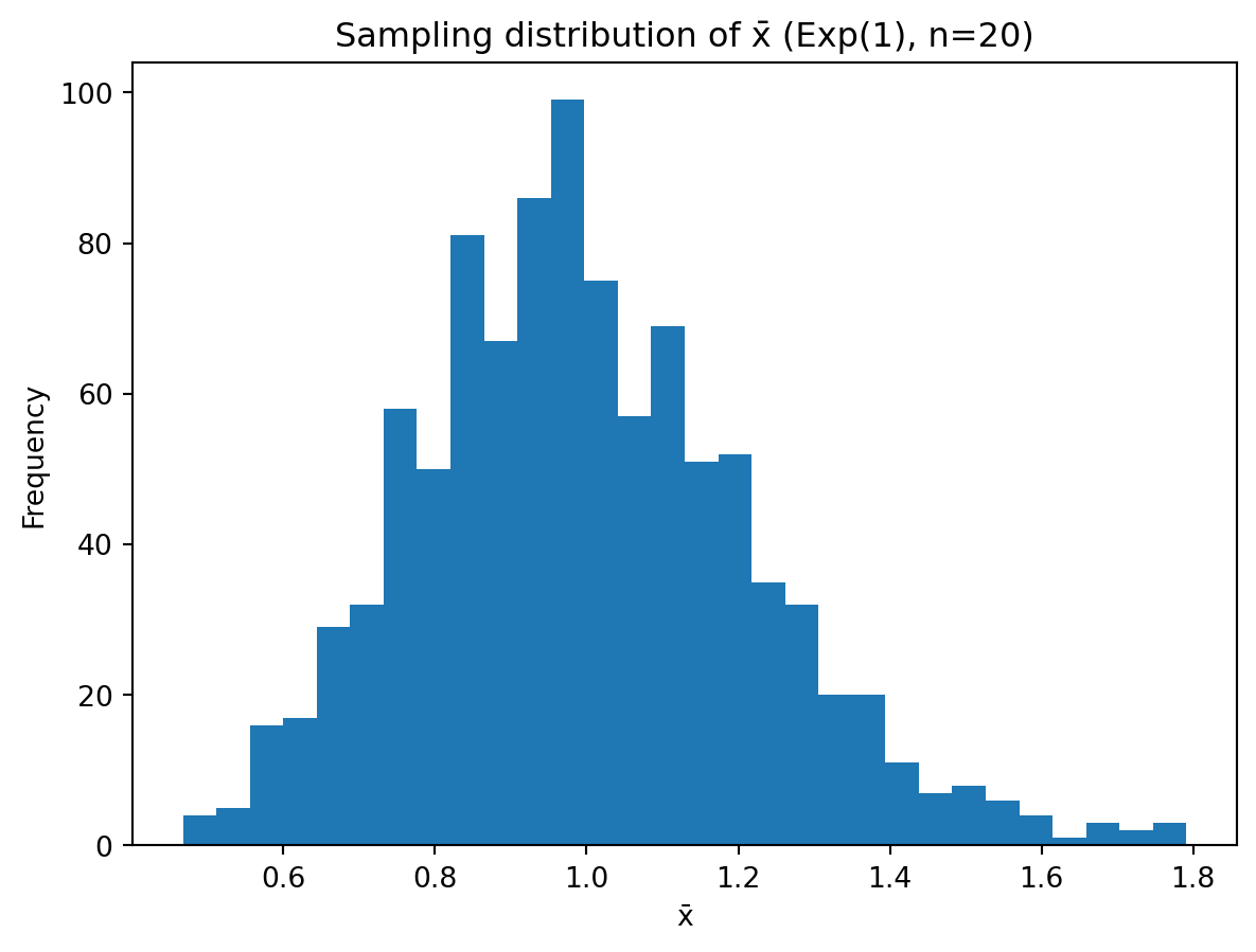
plt.hist(xbar, bins=30)
plt.title("Sampling distribution of x̄ (Exp(1), n=20)")
plt.xlabel("x̄")
plt.ylabel("Frequency")
plt.show()

The histogram looks approximately normal (CLT at work).

mean_xbar = np.mean(xbar)
sd_xbar = np.std(xbar, ddof=1)  # ddof=1 to match R's sd() (sample SD)

mean_theory = 1 / lam
sd_theory = np.sqrt(1 / (lam**2 * n))  # SD of x̄

print(mean_xbar, sd_xbar)
print(mean_theory, sd_theory)
0.9952815150435377 0.22196911266164424
1.0 0.22360679774997896

a,b,c. The simulated mean should be close to 1 (theoretical mean). The simulated SD should be close to theoretical SD calculated by

\[ \sqrt{\frac{1}{n}} = \frac{1}{\sqrt{20}} \approx 0.2236. \]


Exercise 2: Bias of an Estimator

Let \(X_1, X_2, \dots, X_n \sim \text{Uniform}(0,1)\).

Two estimators of the mean \(\mu = 0.5\) are:

\[ \hat{\mu}_1 = \bar{X} \]

and

\[ \hat{\mu}_2 = \frac{n+1}{n}\bar{X}. \]

  1. Simulate 1000 samples with \(n = 10\).
  2. Compute both estimators for each sample.
  3. Calculate the average value of each estimator.

Questions:

  1. Which estimator appears to be unbiased?
  2. Which estimator tends to overestimate the true mean?
  3. How could simulation help compare estimators?
B = 1000
n = 10

# replicate(B, mean(runif(n,0,1)))
xbar = [np.mean(np.random.uniform(0, 1, n)) for _ in range(B)]

mu_hat1 = np.array(xbar)
mu_hat2 = ((n + 1) / n) * mu_hat1

# Compare averages to true mean (0.5)
print(np.mean(mu_hat1), np.mean(mu_hat2))

# Bias
print({
    "bias1": np.mean(mu_hat1) - 0.5,
    "bias2": np.mean(mu_hat2) - 0.5
})

# Histograms
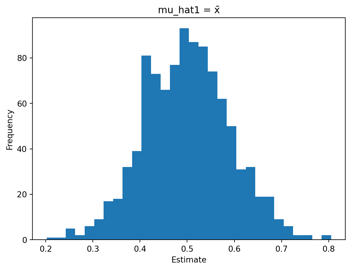
plt.hist(mu_hat1, bins=30)
plt.title("mu_hat1 = x̄")
plt.xlabel("Estimate")
plt.ylabel("Frequency")
plt.show()

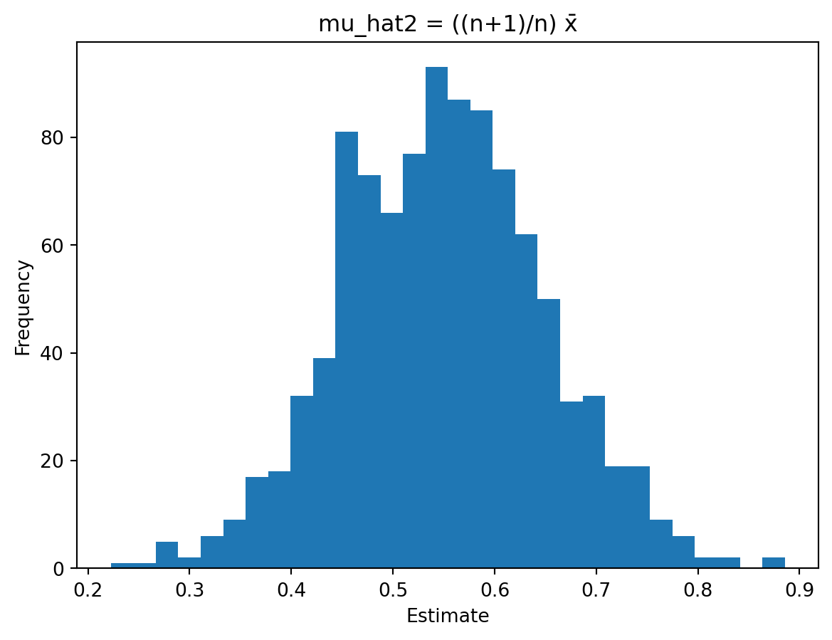
plt.hist(mu_hat2, bins=30)
plt.title("mu_hat2 = ((n+1)/n) x̄")
plt.xlabel("Estimate")
plt.ylabel("Frequency")
plt.show()
0.4994229077830213 0.5493651985613235
{'bias1': np.float64(-0.000577092216978714), 'bias2': np.float64(0.04936519856132349)}

  1. Estimator \(\hat{mu}_1 = \bar{X}\) appears to be unbiased as its average across simulations is very close to 0.5.
  2. Estimator \(\hat{\mu}_2 = \frac{n+1}{n}\bar{X}\) tends to overestimate the true mean as its expected value is 0.55, so it consistently overshoots.
  3. Simulation allows us to:
    • Empirically estimate the bias of each estimator.
    • Compare variability (MSE, variance).
    • Visualise sampling distributions.
    • Understand estimator behaviour without relying solely on algebra.

Exercise 3: MLE for the Bernoulli

Suppose \(X_i \sim \text{Bernoulli}(p)\).

  1. Simulate \(n = 50\) Bernoulli observations with \(p = 0.3\).
  2. Compute the maximum likelihood estimator.
  3. Repeat this simulation 1000 times and record the estimates.

Questions:

  1. Plot a histogram of the 1000 estimates.
  2. What is the mean of the simulated estimates?
  3. Does the estimator appear to be unbiased?
B = 1000
n = 50
p = 0.3

samples = np.random.binomial(1, p, size=(B, n))
p_hat = samples.mean(axis=1)

# Histogram
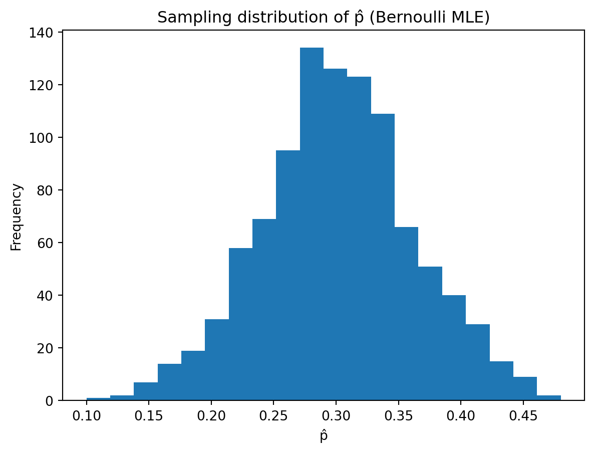
plt.hist(p_hat, bins=20)
plt.title("Sampling distribution of p̂ (Bernoulli MLE)")
plt.xlabel("p̂")
plt.ylabel("Frequency")
plt.show()

print("Mean of p̂:", np.mean(p_hat))   # should be close to 0.3
print("SD of p̂:", np.std(p_hat, ddof=1))  # variability (sample SD like R)

Mean of p̂: 0.30196
SD of p̂: 0.06451294692013627
  1. The histogram looks approximately normal and centred near 0.3.
  2. Mean of the estimates is very close to 0.3.
  3. The estimator appears unbiased as simulation confirms \(E[\hat{p}]=p\).

Exercise 4: MLE for Normal Distribution (Exam-style)

Suppose

\[ X_i \sim N(\mu, \sigma^2), \]

where \(\sigma^2\) is known.

  1. Write down the likelihood function \(L(\mu)\).
  2. Derive the log-likelihood function.
  3. Show that the maximum likelihood estimator of \(\mu\) is \(\bar{X}.\)
  4. Simulate \(n=40\) observations from \(N(5,1)\)
  5. Compute the MLE of \(\mu\).
  6. Repeat the simulation 1000 times and plot the distribution of the estimates.

Questions:

  1. What is the mean of the simulated estimates?
  2. What does this suggest about the estimator?
  3. How does the variability change if the sample size increases?
  1. Likelihood function:

\[ L(\mu) = \prod_{i=1}^n \frac{1}{\sqrt{2\pi\sigma^2}} \exp\!\left\{-\frac{(x_i - \mu)^2}{2\sigma^2}\right\}. \]

  1. The log-likelihood function:

\[ \begin{aligned} \ell(\mu) &= \log L(\mu) \\ &= \sum_{i=1}^n \left[-\frac{1}{2}\log(2\pi\sigma^2)-\frac{(x_i - \mu)^2}{2\sigma^2}\right] \\ &= -\frac{n}{2}\log(2\pi\sigma^2)-\frac{1}{2\sigma^2}\sum_{i=1}^n (x_i - \mu)^2. \end{aligned} \]

  1. MLE:

\[ \frac{\partial \ell(\mu)}{\partial \mu} = -\frac{1}{2\sigma^2} \cdot 2 \sum_{i=1}^n (x_i - \mu)(-1) = \frac{1}{\sigma^2} \sum_{i=1}^n (x_i - \mu) = 0. \]

\[ \Longrightarrow \sum_{i=1}^n x_i = n\mu \quad \Longrightarrow \quad \hat{\mu}_{\text{MLE}} = \bar{X} = \frac{1}{n}\sum_{i=1}^n X_i. \]

  1. Simulate \(n=40\) observations from \(N(5,1)\)
  2. Compute the MLE of \(\mu\).
  3. Repeat the simulation 1000 times and plot the distribution of the estimates.
# Simulate
n = 40
mu_true = 5
sigma = 1  # sd = 1

x = np.random.normal(loc=mu_true, scale=sigma, size=n)

# MLE for mu when sigma^2 known
mu_hat = np.mean(x)
print("Single sample MLE mu_hat:", mu_hat)

# Repeat 1000 times
B = 1000
mu_hats = np.random.normal(mu_true, sigma, size=(B, n)).mean(axis=1)

# Histogram
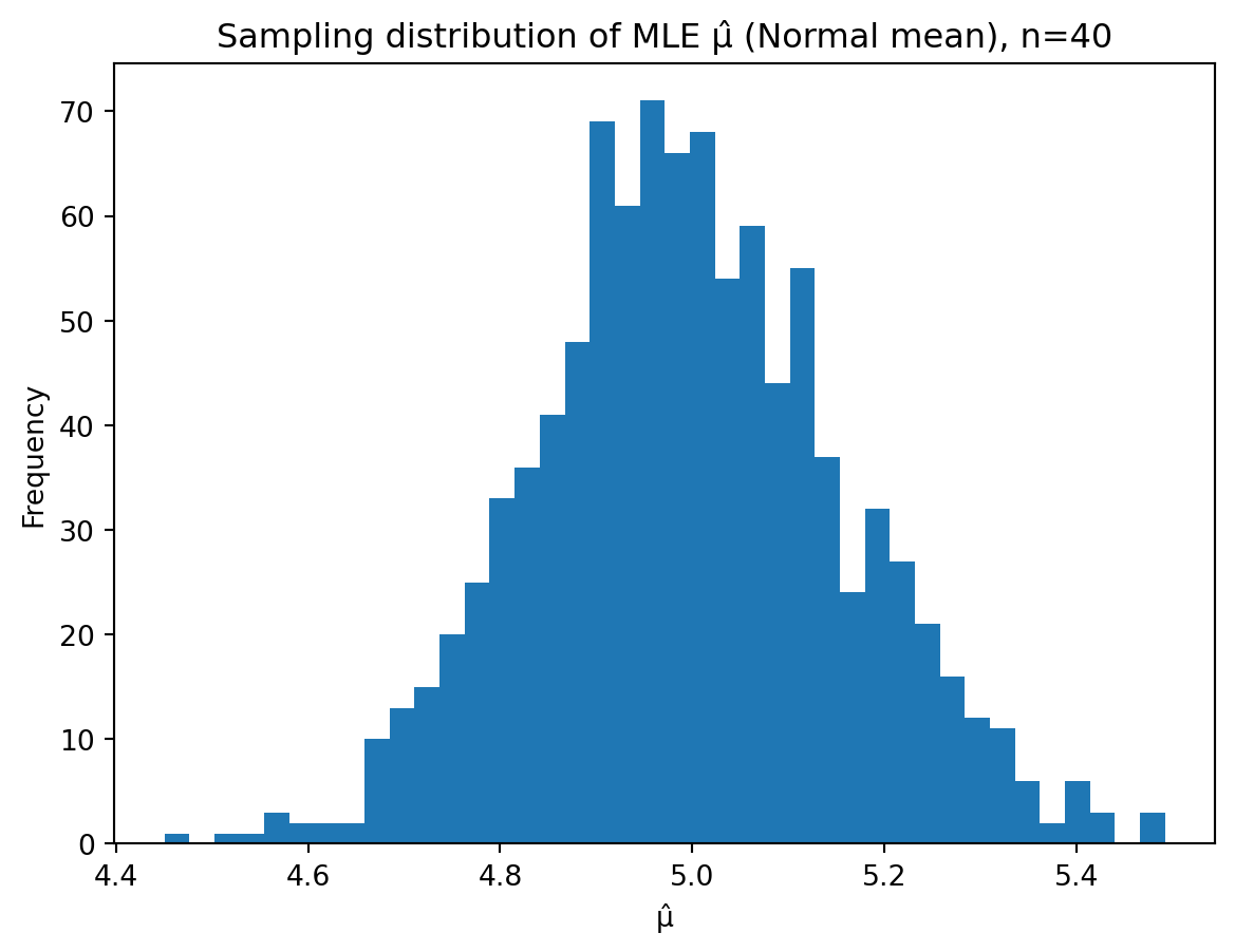
plt.hist(mu_hats, bins=40)
plt.title("Sampling distribution of MLE μ̂ (Normal mean), n=40")
plt.xlabel("μ̂")
plt.ylabel("Frequency")
plt.show()

# Questions a–b
mean_est = np.mean(mu_hats)
sd_est = np.std(mu_hats, ddof=1)  # match R's sd()

print("Mean of estimates:", mean_est)
print("SD of estimates:", sd_est)
Single sample MLE mu_hat: 5.067072305555624

Mean of estimates: 4.995940895656597
SD of estimates: 0.16160063292405424
import pandas as pd

# c. Variability vs sample size
ns = [40, 80, 200]

summary_tbl = pd.DataFrame({
    "n": ns,
    "mean_hat": [np.nan]*len(ns),
    "sd_hat": [np.nan]*len(ns)
})

for i, n_i in enumerate(ns):
    hats = [np.mean(np.random.normal(mu_true, sigma, n_i)) for _ in range(B)]
    hats = np.array(hats)
    
    summary_tbl.loc[i, "mean_hat"] = np.mean(hats)
    summary_tbl.loc[i, "sd_hat"] = np.std(hats, ddof=1)  # match R's sd()

print(summary_tbl)

# Optional: show how sd decreases ~ 1/sqrt(n)
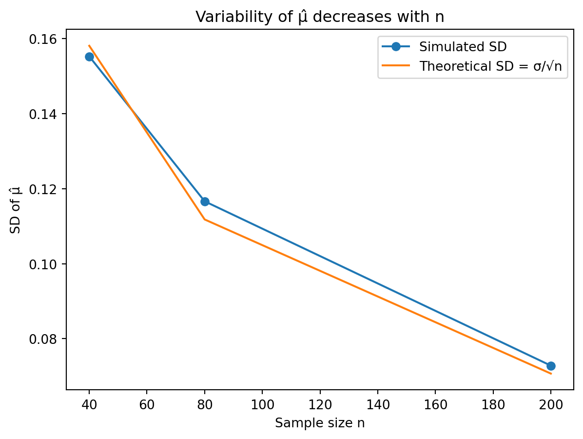
plt.plot(summary_tbl["n"], summary_tbl["sd_hat"], marker="o", label="Simulated SD")
plt.plot(summary_tbl["n"], sigma / np.sqrt(summary_tbl["n"]), label="Theoretical SD = σ/√n")

plt.xlabel("Sample size n")
plt.ylabel("SD of μ̂")
plt.title("Variability of μ̂ decreases with n")
plt.legend()
plt.show()
     n  mean_hat    sd_hat
0   40  5.001451  0.155282
1   80  5.007736  0.116648
2  200  4.998718  0.072831

  1. Mean of the simulated estimates.

The empirical mean of the \(1000\) estimates is \[ \overline{\hat{\mu}} = \frac{1}{1000}\sum_{b=1}^{1000} \hat{\mu}^{(b)}. \] In large simulations, this will be very close to the true value \(5\).

  1. What does this suggest about the estimator?

Since the average of the simulated MLEs is close to \(5\), this suggests that \[ E[\hat{\mu}] = \mu, \]

i.e. \(\hat{\mu} = \bar{X}\) is an unbiased estimator of \(\mu\).

  1. Effect of increasing the sample size on variability.

The variance of \(\bar{X}\) is \[ \operatorname{Var}(\bar{X}) = \frac{\sigma^2}{n}. \]

As \(n\) increases, \(\operatorname{Var}(\bar{X})\) decreases, so the sampling distribution of \(\hat{\mu}\) becomes more concentrated around \(\mu\). In simulation, this appears as a histogram that is more tightly clustered around \(5\) when \(n\) is larger (e.g. \(n=100\) vs. \(n=40\)).


Exercise 5: Confidence Interval for a Mean

Suppose the true distribution is Normal with

\[ \mu = 10, \quad \sigma = 2. \]

  1. Simulate a sample of size \(n = 40\).
  2. Compute the sample mean \(\bar{X}\).
  3. Construct a 95% confidence interval.

Questions:

  1. Does the interval contain the true mean \(\mu = 10\)?
  2. Repeat the experiment 1000 times and record whether the interval contains the true mean.

Compute the proportion of intervals that contain the true mean.

  1. Is this proportion close to 0.95?
  2. What does this illustrate about confidence intervals?
import numpy as np
import matplotlib.pyplot as plt
from statistics import NormalDist

np.random.seed(123)

# Known parameters
mu_true = 10
sigma = 2
n = 40

# 1. Simulate one sample
x = np.random.normal(loc=mu_true, scale=sigma, size=n)

# 2. Sample mean
xbar = np.mean(x)

# 3. 95% confidence interval (sigma known)
z = NormalDist().inv_cdf(0.975)
se = sigma / np.sqrt(n)

CI_lower = xbar - z * se
CI_upper = xbar + z * se

print((CI_lower, CI_upper))

# a. Does the interval contain the true mean?
contains_mu = (mu_true >= CI_lower) and (mu_true <= CI_upper)
print(contains_mu)

# b. Repetition for 1000 simulations
B = 1000
contains = np.zeros(B, dtype=bool)

for b in range(B):
    x = np.random.normal(loc=mu_true, scale=sigma, size=n)
    xbar = np.mean(x)

    CI_lower = xbar - z * se
    CI_upper = xbar + z * se

    contains[b] = (mu_true >= CI_lower) and (mu_true <= CI_upper)

# (b)–(c) Proportion of intervals containing the true mean
prop_contains = np.mean(contains)
print(prop_contains)  # should be close to 0.95

# Optional: visualise sampling variability of xbar
xbars = [np.mean(np.random.normal(mu_true, sigma, n)) for _ in range(B)]

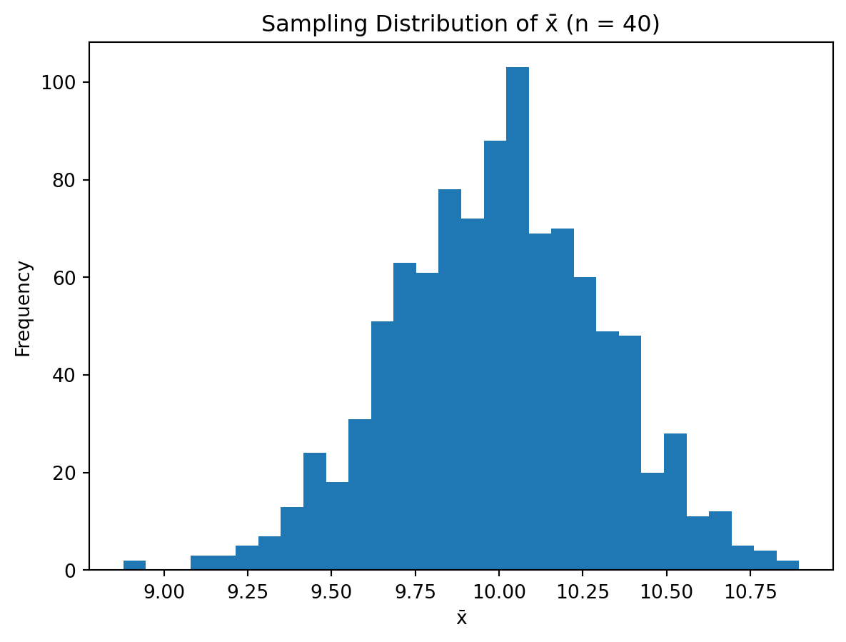
plt.hist(xbars, bins=30)
plt.title("Sampling Distribution of x̄ (n = 40)")
plt.xlabel("x̄")
plt.ylabel("Frequency")
plt.show()
(np.float64(9.213444301221577), np.float64(10.453034365830698))
True
0.936

  1. This simulation illustrates the frequentist coverage interpretation of confidence intervals:
  • A single 95% confidence interval does not guarantee that it contains the true mean.
  • However, if we repeatedly sample from the population and construct a 95% confidence interval each time, then approximately 95% of those intervals will contain the true parameter \(\mu\).
  • Thus, the 95% refers to the long-run proportion of intervals that cover the true parameter, not to a probability statement about any one specific interval.

Part 2: Bayesian inference

Exercise 6: Bayes Theorem

Suppose a test is 95% accurate when a disease is present and 97% accurate when the disease is absent. Suppose that 1% of the population has the disease. Let \(H\) be the event that a disease is present, \(T^+\) be the event of positive test result, and \(T^-\) be the event of negative test result.

  1. Draw a tree diagram or probability table to visualise the conditional probabilities

flowchart LR
    A[Start] --> B{H: Disease?}
    B -->|Yes 1%| C[H]
    B -->|No 99%| D[&sim;H]

    C -->|Test Positive 95%| E[T+ &mid; H]
    C -->|Test Negative 5%| F[T- &mid; H]

    D -->|Test Positive 3%| G[T+ &mid; &sim;H]
    D -->|Test Negative 97%| K[T- &mid; &sim;H]

    linkStyle default stroke:#000,stroke-width:2px

\[ \begin{array}{c|cc} P(T? \mid ?H) & H & \neg H \\ \hline T+ & 95\% & 3\% \\ T- & 5\% & 97\% \\ \hline & 1\% & 99\% \end{array} \]

  1. True positive probability \(P(H \mid T^+)\).

Bayes’ rule:

\[ P(H \mid T^+) = \frac{P(T^+ \mid H)P(H)} {P(T^+ \mid H)P(H) + P(T^+ \mid \neg H)P(\neg H)} \]

Plug in values:

\[ P(H \mid T^+) = \frac{0.95 \cdot 0.01} {0.95 \cdot 0.01 + 0.03 \cdot 0.99} \]

Compute numerator and denominator:

  • Numerator: \(0.0095\)
  • Denominator: \(0.0095 + 0.0297 = 0.0392\)

\[ P(H \mid T^+) = \frac{0.0095}{0.0392} \approx 0.242 \]

True positive probability ≈ 24.2%

Even with a “good” test, the disease is rare, so most positives are false positives.

  1. False positive probability \(P(\neg H \mid T^+)\)

\[ P(\neg H \mid T^+) = 1 - P(H \mid T^+) \]

\[ = 1 - 0.242 = 0.758 \]

False positive probability ≈ 75.8%

  1. True negative probability \(P(\neg H \mid T^-)\)

Bayes’ rule again:

\[ P(\neg H \mid T^-) = \frac{P(T^- \mid \neg H)P(\neg H)} {P(T^- \mid \neg H)P(\neg H) + P(T^- \mid H)P(H)} \]

\[ = \frac{0.97 \cdot 0.99} {0.97 \cdot 0.99 + 0.05 \cdot 0.01} \]

Compute:

  • Numerator: \(0.9603\)
  • Denominator: \(0.9603 + 0.0005 = 0.9608\)

\[ P(\neg H \mid T^-) \approx \frac{0.9603}{0.9608} \approx 0.9995 \]

True negative probability ≈ 99.95%

  1. False negative probability \(P(H \mid T^-)\)

\[ P(H \mid T^-) = 1 - P(\neg H \mid T^-) \]

\[ = 1 - 0.9995 = 0.0005 \]

False negative probability ≈ 0.05%


Exercise 7: Bayesian Estimate

(Albert et al., 2009, Chapter 4, Exercise 4.4)

A woman tells you she can predict the sex of a baby by how high it ‘rides’ in the mothers uterus. ‘High’ means a boy and ‘low’ means a girl. You suspect she is only guessing, but you are not completely sure;

  1. Place a prior distribution on the values of her success rate (\(p\)) in the table below that reflects this belief that she is probably just guessing.
import pandas as pd

x = [
    ["Success rate p", 0, 0.25, 0.5, 0.75, 0.9, 1],
    ["Pr(p) prior",    0, 0.1,  0.75, 0.1,  0.04, 0.01]
]

df = pd.DataFrame(x)
print(df)
                0  1     2     3     4     5     6
0  Success rate p  0  0.25  0.50  0.75  0.90  1.00
1     Pr(p) prior  0  0.10  0.75  0.10  0.04  0.01

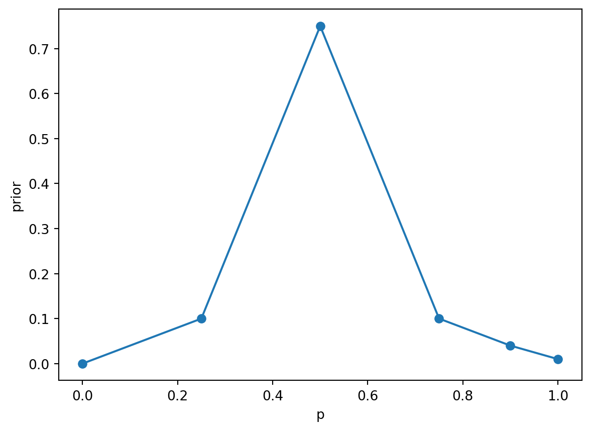
This is a discrete prior with the following pmf \(Pr(p)\):

# Values from the table
p = [0, 0.25, 0.5, 0.75, 0.9, 1]
prior = [0, 0.1, 0.75, 0.1, 0.04, 0.01]

plt.plot(p, prior, marker='o')
plt.xlabel("p")
plt.ylabel("prior")
plt.show()

  1. You conduct an experiment with 10 pregnant women, and the woman is correct 7 times out of 10 in predicting the sex of the unborn baby. Update your probabilities in the table.

This is Binomial data (likelihood):

\[ X \mid p \sim \text{Binomial}(n=10, p) \]

\[ f(X \mid p) = {10\choose X} p^X (1-p)^{10-X} \]

The woman is correct 7 times out of 10 \(\rightarrow X = 7\).

\[ f(X \mid p) = {10\choose 7} p^7 (1-p)^{3} \]

Product:

\[ f(p \mid X) = Pr(p) \times f(X \mid p) \]

Normalising above gives the posterior:

import numpy as np
import pandas as pd
import matplotlib.pyplot as plt
from scipy.stats import binom

p = np.array([0, 0.25, 0.5, 0.75, 0.9, 1])
prior = np.array([0, 0.1, 0.75, 0.1, 0.04, 0.01])

likelihood = binom.pmf(7, 10, p)
product = prior * likelihood
posterior = product / np.sum(product)  # normalise

# Table
x = pd.DataFrame([
    ["Success rate p", *p],
    ["Pr(p) prior", *prior],
    ["Product", *np.round(product, 5)],
    ["Posterior", *np.round(posterior, 5)]
])

print(x.to_string(index=False, header=False))

# Plots
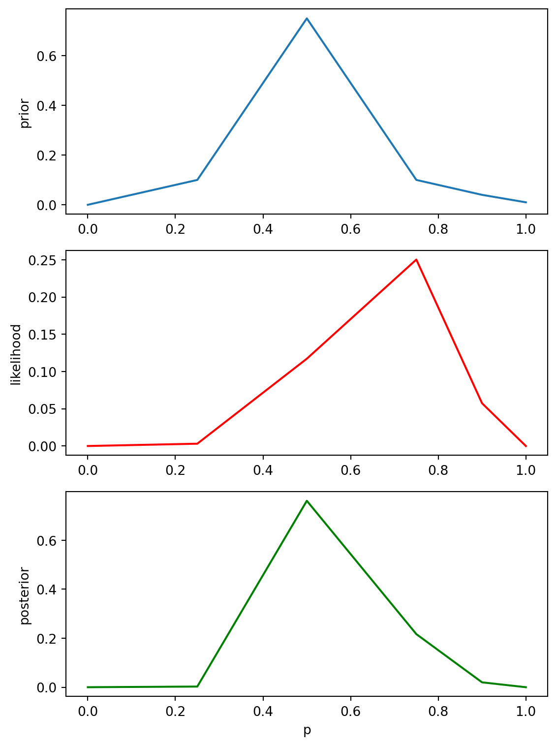
fig, axes = plt.subplots(3, 1, figsize=(6, 8))

axes[0].plot(p, prior)
axes[0].set_ylabel("prior")

axes[1].plot(p, likelihood, color="red")
axes[1].set_ylabel("likelihood")

axes[2].plot(p, posterior, color="green")
axes[2].set_ylabel("posterior")
axes[2].set_xlabel("p")

plt.tight_layout()
plt.show()
Success rate p 0.0 0.25000 0.50000 0.75000 0.90000 1.00
   Pr(p) prior 0.0 0.10000 0.75000 0.10000 0.04000 0.01
       Product 0.0 0.00031 0.08789 0.02503 0.00230 0.00
     Posterior 0.0 0.00267 0.76080 0.21665 0.01987 0.00

  1. Based on the data obtained in part (b) compute the maximum likelihood estimate of \(p\) and place a bound on its estimate.

For a Binomial mode, the MLE is \[ \hat{p}_{\text{MLE}} = \frac{X}{n} = \frac{7}{10} = 0.7. \]

A 95% confidence interval is

\[ \hat{p} \pm 1.96 \sqrt{\frac{\hat{p}(1-\hat{p})}{n}} \approx 0.7 \pm 0.28, \]

so roughly (0.42, 0.98).

  1. How likely is she to have some skill in gender prediction? How likely is she to be just guessing?

Let’s define

  • Just guessing: \(p = 0.5\).
  • Some skill: \(p > 0.5, \quad p \in \{0.75, 0.9, 1\}\).

From the posterior:

\[ Pr(p=0.5 \mid X) \approx 0.7608 \]

\[ Pr(p>0.5 \mid X) \approx 0.2167 + 0.0199 \approx 0.2366 \]

  • About 76% chance she’s just guessing.
  • About 24% chance she has some real skill.

The data nudges you toward “maybe some skill,” but your prior belief that she’s guessing still dominates.

  1. Repeat (b) and (d) with a flat prior on p. 
from scipy.stats import binom

p = np.array([0, 0.25, 0.5, 0.75, 0.9, 1])

# Uniform prior (1/6 each)
prior1 = np.repeat(1/6, 6)

# Likelihood dbinom(7,10,p)
likelihood = binom.pmf(7, 10, p)

# Posterior
posterior = (prior1 * likelihood) / np.sum(prior1 * likelihood)

# Table
x1 = pd.DataFrame([
    ["Success rate p", *p],
    ["Pr(p) prior", *np.round(prior1, 4)],
    ["Likelihood", *np.round(likelihood, 4)],
    ["Posterior", *np.round(posterior, 4)]
])

print(x1.to_string(index=False, header=False))
Success rate p 0.0000 0.2500 0.5000 0.7500 0.9000 1.0000
   Pr(p) prior 0.1667 0.1667 0.1667 0.1667 0.1667 0.1667
    Likelihood 0.0000 0.0031 0.1172 0.2503 0.0574 0.0000
     Posterior 0.0000 0.0072 0.2738 0.5848 0.1341 0.0000

\[ Pr(p=0.5 \mid X) \approx 0.2738 \]

\[ Pr(p>0.5 \mid X) \approx 0.5848 + 0.1341 \approx 0.7189 \]

  • About 27% chance she’s just guessing.
  • About 72% chance she has some real skill.

With a flat prior, the same data makes “some skill” the more plausible story.

Important

Same likelihood, different priors → different posterior stories.

Exercise 8: Conjugate Prior

Suppose the number of customers arriving at a service desk in one hour follows a Poisson distribution with unknown rate \(\lambda\):

\[ X_i \sim \text{Poisson}(\lambda), \quad i = 1, \dots, n. \]

A prior distribution is placed on \(\lambda\):

\[ \lambda \sim \text{Gamma}(\alpha, \beta), \]

where \(\alpha > 0\) and \(\beta > 0\).

Assume the prior parameters are

\[ \alpha = 3, \qquad \beta = 1. \]

During five observed hours, the number of arriving customers is recorded as

\[ 8,\; 6,\; 7,\; 9,\; 10. \]

Questions:

  1. Write down the likelihood function for \(\lambda\) based on the observed data.
  2. Using the conjugacy of the Gamma prior with the Poisson likelihood, determine the posterior distribution of \(\lambda\). Specify the updated parameters of the Gamma distribution.
  3. Compute the posterior mean of \(\lambda\).
  4. Find the maximum likelihood estimator (MLE) of \(\lambda\) based on the observed data. Compare the MLE with the posterior mean and briefly comment on the difference.
  5. Using statistical software (R or Python), compute a 95% credible interval for \(\lambda\) from the posterior distribution.

Hint:

For the Gamma distribution parameterised as \(\text{Gamma}(\alpha, \beta)\) with shape \(\alpha\) and rate \(\beta\): \[ E[\lambda] = \frac{\alpha}{\beta}. \]

For the Gamma–Poisson conjugate model, the posterior parameters are

\[ \alpha_{\text{post}} = \alpha + \sum x_i, \]

\[ \beta_{\text{post}} = \beta + n. \]

  1. Likelihood function

Given data \(x_1, \dots, x_n\) with \(x_i \sim \text{Poisson}(\lambda)\) independently, the likelihood is
\[ L(\lambda \mid x_1,\dots,x_n) = \prod_{i=1}^n \frac{e^{-\lambda}\lambda^{x_i}}{x_i!} = e^{-n\lambda}\lambda^{\sum_{i=1}^n x_i} \prod_{i=1}^n \frac{1}{x_i!}. \]

For the specific data \(8,6,7,9,10\) with \(n=5\) and \(\sum x_i = 40\), \[ L(\lambda \mid \mathbf{x}) \propto e^{-5\lambda}\lambda^{40}. \]

  1. Posterior distribution

Prior: \(\lambda \sim \text{Gamma}(\alpha,\beta)\) with \(\alpha=3\), \(\beta=1\).

Using conjugacy: \[ \alpha_{\text{post}} = \alpha + \sum x_i = 3 + 40 = 43, \] \[ \beta_{\text{post}} = \beta + n = 1 + 5 = 6. \]

So the posterior is \[ \lambda \mid \mathbf{x} \sim \text{Gamma}(43, 6). \]

  1. Posterior mean

For \(\lambda \sim \text{Gamma}(\alpha_{\text{post}}, \beta_{\text{post}})\), \[ E[\lambda \mid \mathbf{x}] = \frac{\alpha_{\text{post}}}{\beta_{\text{post}}} = \frac{43}{6} \approx 7.1667. \]

  1. MLE of \(\lambda\) and comparison

For Poisson data, the MLE is the sample mean: \[ \hat{\lambda}_{\text{MLE}} = \bar{x} = \frac{8+6+7+9+10}{5} = \frac{40}{5} = 8. \]

Comparison:

  • MLE: \(\hat{\lambda}_{\text{MLE}} = 8\)
  • Posterior mean: \(E[\lambda \mid \mathbf{x}] = 43/6 \approx 7.17\)

The posterior mean is shrunk toward the prior mean
\[ E[\lambda] = \frac{\alpha}{\beta} = \frac{3}{1} = 3, \] reflecting prior information plus data, whereas the MLE uses only the data.

  1. 95% credible interval in R

Posterior: \(\lambda \mid \mathbf{x} \sim \text{Gamma}(43, 6)\).

A 95% credible interval is given by the 2.5% and 97.5% quantiles:

from scipy.stats import gamma

alpha_post = 43
beta_post = 6   # rate

# Posterior mean
post_mean = alpha_post / beta_post
print(post_mean)

# 95% credible interval
# SciPy uses scale = 1 / rate
ci_lower = gamma.ppf(0.025, a=alpha_post, scale=1/beta_post)
ci_upper = gamma.ppf(0.975, a=alpha_post, scale=1/beta_post)

print((ci_lower, ci_upper))
7.166666666666667
(np.float64(5.18655220199453), np.float64(9.461966463081774))

This returns a 95% credible interval of the form
\[ [\lambda_{0.025},\; \lambda_{0.975}] = [5.1866, 9.4620]. \]

Extra Exercises

  1. Let \(X_1, X_2, \dots, X_n\) have a joint density function \(f(X_1, X_2, \dots, X_n \mid \theta)\). Given \(X_1 = x_1, X_2 = x_2, \dots, X_n = x_n\) is observed, the function of \(\theta\) defined by

\[ L(\theta) = L(\theta \mid x_1, x_2, \dots, x_n) = f(x_1, x_2, \dots, x_n \mid \theta) \]

  is the likelihood function.

  In the following questions you are asked to specify the likelihood functions for given scenarios.

  1. A coin is flipped 100 times. Given that there were 55 heads, specify the likelihood function for \(\theta\), the probability of heads on a single toss.

\[ L(\theta) = {100 \choose 55}\theta^55 (1-\theta)^{100-55} \]

  1. Consider the distribution \(\text{Multinomial}(n = 6, \theta, \theta, 1 - 2\theta)\). The following two samples are drawn from this distribution: \(X = (1,3,2)\) and \(X = (2,2,2)\). Specify the likelihood function for each sample and compare them.

\[ \begin{aligned} L(\theta \mid 1,3,2) &= \frac{6!}{1!\,3!\,2!}\,\theta^{1}\theta^{3}(1-2\theta)^{2} \\ &= \frac{6!}{1!\,3!\,2!}\,\theta^{4}(1-2\theta)^{2} \\ &\propto \theta^{4}(1-2\theta)^{2} \end{aligned} \]

\[ \begin{aligned} L(\theta \mid 2,2,2) &= \frac{6!}{2!\,2!\,2!}\,\theta^{2}\theta^{2}(1-2\theta)^{2} \\ &= \frac{6!}{2!\,2!\,2!}\,\theta^{4}(1-2\theta)^{2} \\ &\propto \theta^{4}(1-2\theta)^{2} \end{aligned} \]

Both have the same mathematical form.

  1. An actuary has been advised to use the following claim size distribution as a model for a particular type of claim, with claim sizes measured in units of A$100,

\[ f_X(x) = \frac{x^2}{2\theta^3} e^{-x/\theta}, \qquad 0 < x < \infty, \quad \theta > 0 \]

  Let \(x_1, x_2, \dots, x_n\) be a random sample of \(n\) claim sizes for such claims. Specify the likelihood function and the log-likelihood function.

\[ \begin{aligned} L(\theta) &= \prod_{i=1}^{n} f_X(x_i) \\ &= \prod_{i=1}^{n} \frac{x_i^2}{2\theta^3} \exp\!\left(-\frac{x_i}{\theta}\right) \\ &= \left( \frac{x_1^2}{2\theta^3} e^{-x_1/\theta} \right) \left( \frac{x_2^2}{2\theta^3} e^{-x_2/\theta} \right) \cdots \left( \frac{x_n^2}{2\theta^3} e^{-x_n/\theta} \right) \\ &= \frac{\displaystyle \prod_{i=1}^{n} x_i^2 \; \exp\!\left( -\sum_{i=1}^{n} \frac{x_i}{\theta} \right)} {2^n \theta^{3n}} \end{aligned} \]

\[ \begin{aligned} \ln(L(\theta)) &= \ln\!\left( \frac{\prod_{i=1}^{n} x_i^{2}\, e^{-\sum_{i=1}^{n} x_i/\theta}} {2^{n}\theta^{3n}} \right) \\[6pt] &= \ln\!\left(\prod_{i=1}^{n} x_i^{2} e^{-\sum_{i=1}^{n} x_i/\theta}\right) - \ln(2^{n}\theta^{3n}) \\[6pt] &= \sum_{i=1}^{n} \ln(x_i^{2}) - \sum_{i=1}^{n} \frac{x_i}{\theta} - n\ln(2) - 3n\ln(\theta) \\[6pt] &\propto -\sum_{i=1}^{n} \frac{x_i}{\theta} - 3n\ln(\theta) \end{aligned} \]

  1. Consider a sample of 1000 motor insurance policies. We assume that the annual total claim amounts per policy are independent and identically distributed. We denote by \(X\) the number of policies with a total amount of over A$5000 claimed in a calendar year, and assume that \(X\) has a Binomial distribution with parameters \(n = 1000\) and \(p\). An analyst wishes to estimate the unknown proportion \(p\) of claims with amount greater than A$5000 per year.
  1. Derive the maximum likelihood estimator for \(p\).

\[ \begin{aligned} l(p) &= k\, p^{x}(1-p)^{\,n-x} \\[6pt] \frac{\partial l(p)}{\partial p} &= \frac{x}{p} - \frac{n-x}{1-p} \\[6pt] \frac{\partial^{2} l(p)}{\partial p^{2}} &= \frac{x}{p^{2}} - \frac{n-x}{(1-p)^{2}} < 0 \\[6pt] \hat{p} &= \frac{x}{n} \end{aligned} \]

  1. Derive the Bayesian estimator of \(p\) under quadratic loss assuming that the prior distribution of \(p\) is beta with parameters \(\alpha\) and \(\beta\) respectively.

\[ \begin{aligned} \pi(p) &\propto p^{x}(1-p)^{\,n-x}\, p^{\alpha-1}(1-p)^{\beta-1} \\[6pt] &\propto p^{\,x+\alpha-1}(1-p)^{\,n-x+\beta-1} \\[6pt] &\sim \mathrm{Beta}(x+\alpha,\; n-x+\beta) \\[6pt] &\sim \mathrm{Beta}(x+\alpha,\; 1000-x+\beta) \end{aligned} \]

\[ \begin{aligned} \hat{p} &= \mathbb{E}[p \mid x] = \frac{x+\alpha}{n+\alpha+\beta} = \frac{x+\alpha}{1000+\alpha+\beta} \end{aligned} \]

  1. Comment on the relationship between the prior distribution and the posterior distribution of \(p\) obtained in (b).

Conjugate prior, same form of prior and posterior distribution.

  1. Assume that 50 out of 1000 policies in an actual sample have a total claim amount of over A$5000.
  • Estimate \(p\) using the MLE. \[ \hat{p} = 50/1000 = 0.05 \]
  • Estimate \(p\) using the Bayesian estimator under quadratic loss, given that the parameters of the beta prior distribution are \(\alpha = 2\) and \(\beta = 2\) respectively. \[ \hat{p} = (50+2)/(1000+4) = 0.0518 \]
  • Comment on the difference between the values estimated in MLE and Bayesian Estimate.

The two estimators are the same.

  1. While travelling through the Mushroom Kingdom, Mario and Luigi find some rather unusual coins. They agree on a prior of \(f(\theta) \sim \text{Beta}(5,5)\) for the probability of heads, though they disagree on what experiment to run to investigate \(\theta\) further.

    • Mario decides to flip a coin 5 times. He gets four heads in five flips.
    • Luigi decides to flip a coin until the first tails. He gets four heads before the first tail.

  Show that Mario and Luigi will arrive at the same posterior on \(\theta\), and calculate this posterior.
Mario

Prior is Beta(5,5):

\[ f(\theta) = \frac{\theta^4(1-\theta)^4}{B(5,5)} \]

Likelihood is Binomial(5, \(\theta\)):

\[ f(X \mid \theta) = {5 \choose 4}\theta^4(1-\theta)^1 \]

Posterior:

\[ \begin{aligned} f(\theta \mid X) &\propto \theta^8 (1-\theta)^5 \\ &\propto \theta^{9-1} (1-\theta)^{6-1} \\ &\sim \text{Beta}(9,6). \end{aligned} \]

Luigi

Prior is Beta(5,5):

\[ f(\theta) = \frac{\theta^4(1-\theta)^4}{B(5,5)} \]

Likelihood is Geometric(\(\theta\)):

\[ f(X \mid \theta) = \theta^4(1-\theta)^1 \]

Posterior:

\[ \begin{aligned} f(\theta \mid X) &\propto \theta^8 (1-\theta)^5 \\ &\propto \theta^{9-1} (1-\theta)^{6-1} \\ &\sim \text{Beta}(9,6). \end{aligned} \]

Both arrive at the same pposterior Beta(9, 5).