43  Markov Chain Monte Carlo

In the previous chapter, we saw how to use Monte Carlo simulation to estimate integrals. In this chapter, we will see how to use Markov Chain Monte Carlo (MCMC) methods to sample from complicated probability distributions. This is a powerful technique that is widely used in statistics, machine learning, and many other fields.

Specifically, we will focus on a MCMC algorithm: Gibbs sampling. We will also see how to use this algorithm to perform Bayesian inference, which is a powerful framework for statistical modeling and inference.

43.1 Gibbs Sampling

In many statistical applications, especially Bayesian inference, we are interested in sampling from a complicated multivariate distribution.

Suppose we wish to sample from the joint distribution

\[ p(x,y), \]

or more generally,

\[ p(x_1,x_2,\dots,x_d). \]

In practice, direct sampling (as in Multivariate Simulation) from the full joint distribution may be extremely difficult or even impossible.

However, the corresponding conditional distributions are often much easier to work with.

For example, we may know how to sample from

\[ p(x|y) \quad \text{and} \quad p(y|x), \]

even though sampling directly from \(p(x,y)\) is difficult.

The Gibbs sampler exploits this idea.

Instead of sampling all variables simultaneously, Gibbs sampling repeatedly samples each variable conditional on the current values of the others.

This produces a Markov chain whose long-run distribution converges to the desired target distribution.

Suppose we want to sample from a joint distribution

\[ p(x,y). \]

The Gibbs sampler alternates between the two conditional distributions:

1. sample a new value of \(x\) conditional on the current value of \(y\);
2. sample a new value of \(y\) conditional on the updated value of \(x\).

The iterative updates are:

\[ x^{(t+1)} \sim p(x|y^{(t)}), \]

\[ y^{(t+1)} \sim p(y|x^{(t+1)}). \]

These updates are repeated many times.

The sequence of samples forms a Markov chain.

After sufficiently many iterations, the chain behaves as though it were sampling from the target joint distribution.

TipWhy Gibbs Sampling Works

The Gibbs sampler constructs a Markov chain with the target distribution as its stationary distribution.

The key intuition is:

• each update uses the correct conditional distribution;
• repeated conditional updating gradually explores the full joint distribution;
• dependence between variables is captured automatically through the iterative updates.

Unlike ordinary Monte Carlo simulation:

• samples are not independent;
• each sample depends on the previous state of the chain.

This dependence is the defining feature of Markov chain Monte Carlo (MCMC).

Gibbs Sampling Algorithm

Suppose the target distribution is multivariate with \(d\) variables:

\[ p(x_1,x_2,\dots,x_d). \]

Step 1 — Choose initial values

Select starting values:

\[ x_1^{(0)},x_2^{(0)},\dots,x_d^{(0)}. \]

Step 2 — Sequential conditional updates

For iteration \(t=0,1,2,\dots\),

Update each variable one at a time:

\[ x_1^{(t+1)} \sim p(x_1|x_2^{(t)},x_3^{(t)},\dots,x_d^{(t)}), \]

\[ x_2^{(t+1)} \sim p(x_2|x_1^{(t+1)},x_3^{(t)},\dots,x_d^{(t)}), \]

and so on until

\[ x_d^{(t+1)} \sim p(x_d|x_1^{(t+1)},\dots,x_{d-1}^{(t+1)}). \]

The Gibbs sampler updates one variable at a time, conditional on the current values of all the other \(d−1\) variables.

Step 3 — Repeat

Repeat for many iterations.

The generated sequence approximates samples from the target distribution.

NoteGibbs Sampling and Markov Chains

The Gibbs sampler is an example of a Markov process.

Recall from Stochastic Modelling chapter,

a Markov process depends only on the current state, not the full history.

In Gibbs sampling:

• the next sample depends only on the current values of the variables;
• previous iterations influence the future only through the current state.

Thus, the Gibbs sampler naturally fits into the broader framework of stochastic processes and Markov chains.

Example 1: Bivariate Normal

Consider the bivariate normal distribution:

\[ \begin{pmatrix} X \\ Y \end{pmatrix} \sim N\left( \begin{pmatrix} 0 \\ 0 \end{pmatrix}, \begin{pmatrix} 1 & \rho \\ \rho & 1 \end{pmatrix} \right). \]

Suppose \(\rho = 0.8\). Use Gibbs sampling to generate samples from this distribution.

Step 0 — Identify conditional distributions

Recall from Multivariate Distribution, the joint density can be written as

\[ f(x,y)= \frac{1}{2\pi\sqrt{1-\rho^2}} \exp\left( -\frac{1}{2(1-\rho^2)} (x^2 - 2\rho xy + y^2) \right). \]

To obtain the conditional distribution of \(X\mid Y= y\), we can treat \(y\) as a constant and view the joint density as a function of \(x\) alone. This gives

\[ f(x|y) \propto \exp\left( -\frac{1}{2(1-\rho^2)} (x^2 - 2\rho xy) \right). \]

Now complete the square in \(x\):

\[ x^2 - 2\rho xy = (x-\rho y)^2 - \rho^2 y^2. \]

Substituting this into the exponent gives

\[ f(x|y) \propto \exp\left( -\frac{(x-\rho y)^2}{2(1-\rho^2)} \right). \]

This is the kernel of a normal distribution¹ with mean \(\mathbb{E}[X|Y=y] = \rho y\) and variance \(\text{Var}(X|Y=y) = 1-\rho^2\).

Thus,

\[ \boxed{X|Y=y \sim N(\rho y,1-\rho^2)} \]

Similarly, \[ \boxed{Y|X=x \sim N(\rho x,1-\rho^2)} \]

NoteInterpretation of Conditional Distributions

The conditional distributions reveal several key properties of the bivariate normal distribution:

• \(X\) and \(Y\) are positively correlated (since \(\rho > 0\));
• the mean of \(X\) given \(Y\) is proportional to \(Y\), and vice versa;
• the variance of each conditional distribution is reduced compared to the marginal variance², reflecting the information gained from conditioning on the other variable.

From this, we can write down the Gibbs sampling algorithm for this bivariate normal distribution:

1. Choose initial values \(X^{(0)}\) and \(Y^{(0)}\).

2. sample \(X\) given current \(Y\) and sample \(Y\) given updated \(X\): \[X^{(t+1)} \sim N(\rho Y^{(t)}, 1-\rho^2)\] \[Y^{(t+1)} \sim N(\rho X^{(t+1)}, 1-\rho^2)\]

3. repeat

TipVisualising Gibbs Sampling - Bivariate Normal Case

Figure 43.1: Bivariate Gibbs Sampling

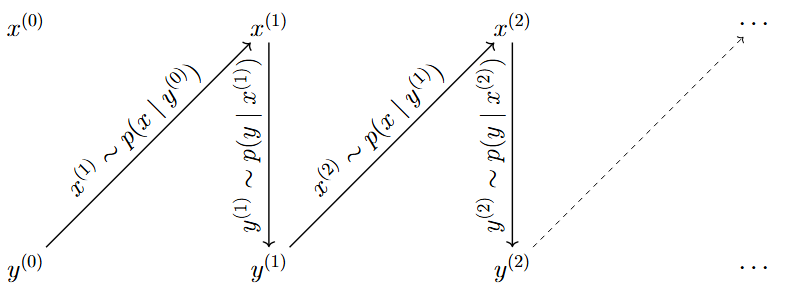
Figure Figure 43.1 illustrates the Gibbs sampling mechanism for a bivariate distribution. Starting from an initial point \((x_0, y_0)\), the sampler first updates \(x\) conditional on the current value of \(y\). Then \(y\) is updated conditional on the newly updated \(x\). Repeating this alternating procedure generates a Markov chain that gradually explores the target joint distribution. Since only one coordinate is updated at a time, the Gibbs sampler typically moves through the state space in a zig-zag pattern.

Analytical Example of Gibbs Sampling Iterations

From the setup, we have

\[ \rho = 0.8, \qquad 1-\rho^2 = 1-0.8^2 = 0.36. \]

Therefore, each conditional distribution has standard deviation

\[ \sqrt{1-\rho^2} = \sqrt{0.36} = 0.6. \]

Step 1 — Choose initial values

\[ X^{(0)} = 3, \qquad Y^{(0)} = -3. \]

Step 2 & 3 — Update variables and repeat

• At iteration \(t=0\),

  we first update \(X\) using the current value \(Y^{(0)}=-3\):

\[ X^{(1)} \sim N(0.8Y^{(0)},0.36) = N(-2.4,0.36). \]

  Randomly draw a value from this distribution:

x1 <- rnorm(1, mean = 0.8 * (-3), sd = sqrt(0.36))
x1 <- round(x1, 2); x1

[1] -2.43

  \(\therefore X^{(1)} = -2.43.\) Now update \(Y\) using the newly updated value \(X^{(1)}\):

\[ Y^{(1)} \sim N(0.8X^{(1)},0.36) = N(-1.944,0.36). \]

  Randomly draw a value from this distribution:

y1 <- rnorm(1, mean = 0.8 * x1, sd = sqrt(0.36))
y1 <- round(y1, 2); y1

[1] -1.84

  \(\therefore Y^{(1)} = -1.84.\) Thus, after the first iteration, we have

\[ \boxed{(X^{(1)},Y^{(1)}) = (-2.43,-1.84)}. \]

• At iteration \(t=1\),

  we repeat the same process. First update \(X\) using \(Y^{(1)}=-1.84\):

\[ X^{(2)} \sim N(0.8Y^{(1)},0.36) = N(-1.472,0.36). \]

  Randomly draw a value from this distribution:

x2 <- rnorm(1, mean = 0.8 * y1, sd = sqrt(0.36))
x2 <- round(x2, 2); x2

[1] -1.44

  \(\therefore X^{(2)} = -1.44.\) Now update \(Y\) using the newly updated value \(X^{(2)}\):

\[ Y^{(2)} \sim N(0.8X^{(2)},0.36) = N(-1.152,0.36) \]

  Randomly draw a value from this distribution:

y2 <- rnorm(1, mean = 0.8 * x2, sd = sqrt(0.36))
y2 <- round(y2, 2); y2

[1] -0.98

Thus,

\[ \boxed{(X^{(2)},Y^{(2)})=(-1.44,-0.98)}. \]

By repeating this process for many iterations, we generate a sequence of samples that approximates the target bivariate normal distribution.

Code Example of Gibbs Sampling Iterations

set.seed(1234)

n <- 5000
rho <- 0.8
sd_cond <- sqrt(1 - rho^2)

x <- numeric(n)
y <- numeric(n)

x[1] <- 0
y[1] <- 0

for(i in 2:n){
  x[i] <- rnorm(1, mean = rho * y[i-1], sd = sd_cond)

  y[i] <- rnorm(1, mean = rho * x[i], sd = sd_cond)
}

plot(x, y, pch = 16, cex = 0.4, col = rgb(0,0,1,0.3),
     xlab = "X", ylab = "Y", main = "Gibbs Samples from a Bivariate Normal")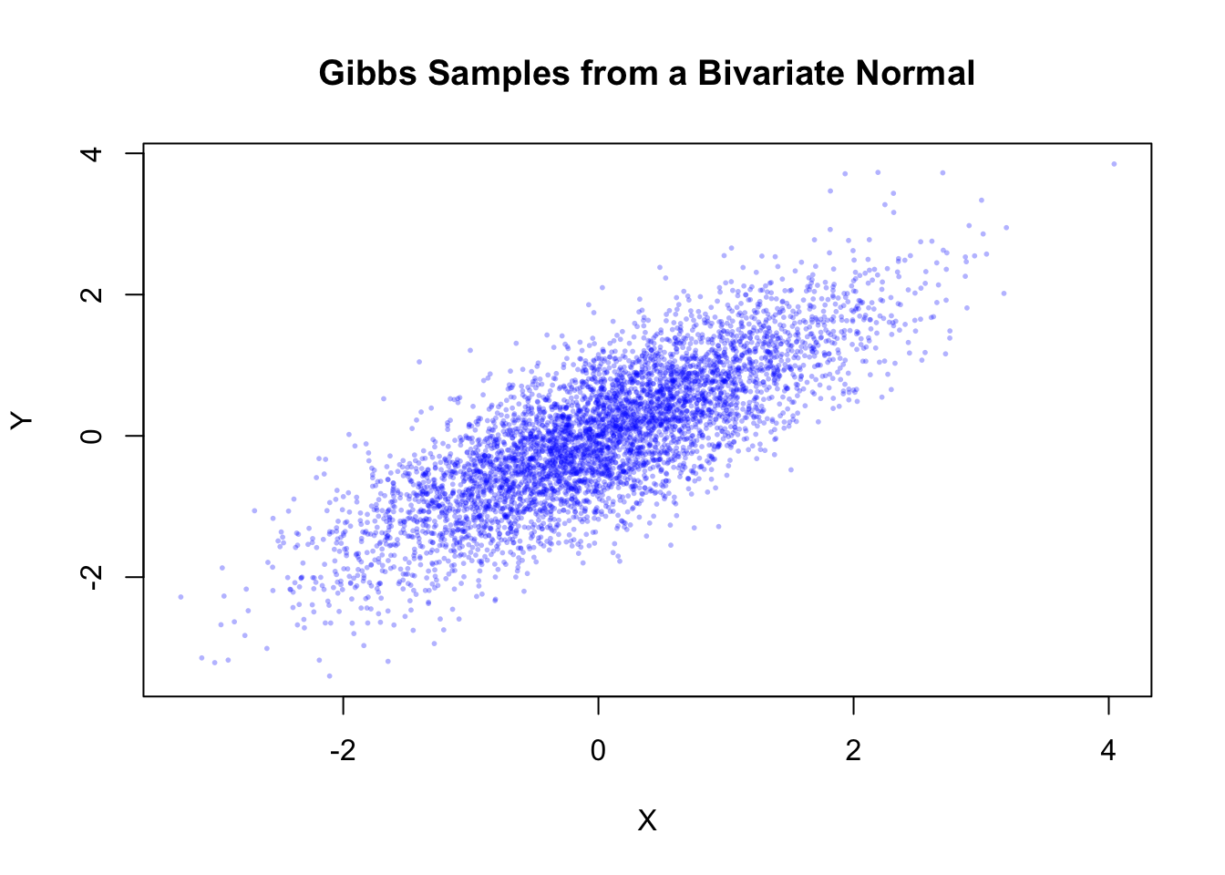

import numpy as np
import matplotlib.pyplot as plt

np.random.seed(1234)
n = 5000
rho = 0.8
sd_cond = np.sqrt(1 - rho**2)
x = np.zeros(n)
y = np.zeros(n)
x[0] = 0
y[0] = 0
for i in range(1, n):
    x[i] = np.random.normal(loc=rho * y[i-1], scale=sd_cond)
    y[i] = np.random.normal(loc=rho * x[i], scale=sd_cond)

plt.scatter(x, y, alpha=0.3)
plt.xlabel("X")
plt.ylabel("Y")
plt.title("Gibbs Samples from a Bivariate Normal")
plt.show()

The simulated points approximate the target bivariate normal distribution. Although the samples are generated one coordinate at a time, the collection of points eventually reproduces the elliptical shape and positive dependence of the target bivariate normal distribution.

NoteConnection to Previous Chapter: Multivariate Simulation

In the Multivariate Simulation chapter, we generated dependent random variables using techniques such as:

• linear transformations and Cholesky decomposition for multivariate normal simulation;
• copulas for modelling more general dependence structures.

Those approaches are examples of direct simulation methods: we can generate samples from the joint distribution directly using known transformations.

Gibbs sampling is different. Instead of sampling directly from the joint distribution, Gibbs sampling generates samples indirectly through a sequence of conditional distributions. This becomes particularly useful when:

• the joint distribution is difficult to sample from directly;
• no convenient transformation is available;
• the distribution is only known up to a proportionality constant (common in Bayesian statistics).

Thus, Gibbs sampling extends simulation methods to settings where direct multivariate simulation is no longer feasible.

Example 2: Multivariate Normal

Let

\[ (X_1, X_2, X_3)^T \sim N\left(\mathbf{0}, \Sigma\right), \]

where

\[ \Sigma = \begin{pmatrix} 1 & 0.8 & 0.5 \\ 0.8 & 1 & 0.3 \\ 0.5 & 0.3 & 1 \end{pmatrix}. \]

Use Gibbs sampling to generate samples from this distribution.

Step 0 — Identify conditional distributions

For a multivariate normal distribution, the conditional distribution of one component given the others is also normal.

Partition the random vector as \(X_j\) and \(X_{-j}\). Then

\[ X_j \mid X_{-j}=x_{-j} \sim N(\mu_{j|-j},\sigma^2_{j|-j}), \]

where

\[ \mu_{j|-j} = \mu_j + \Sigma_{j,-j} \Sigma_{-j,-j}^{-1} (x_{-j}-\mu_{-j}), \]

and

\[ \sigma^2_{j|-j} = \Sigma_{jj} - \Sigma_{j,-j} \Sigma_{-j,-j}^{-1} \Sigma_{-j,j}. \]

In this example, \(\mu=\mathbf 0\), so the conditional means simplify to linear combinations of the remaining variables.

TipVisualising Gibbs Sampling - Multivariate Normal Case

Figure 43.2: Multivariate Gibbs Sampling

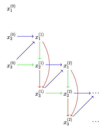
Figure Figure 43.2 illustrates the Gibbs sampler for a three-dimensional distribution. Blue, green, and red arrows represent the conditional dependencies used when updating x1, x2, and x3, respectively. Each update uses the most recently available coordinate values, producing a sequential coordinate-wise Markov chain. Since only one coordinate is updated at a time, the Gibbs sampler typically moves through the state space in a staircase pattern.

Step 1 — Choose initial values

Choose a starting point, for example

\[ (X_1^{(0)},X_2^{(0)},X_3^{(0)})=(3,-3,2). \]

Step 2 — Update one coordinate at a time

At iteration \(t\), update:

\[ X_1^{(t+1)} \sim p(X_1\mid X_2^{(t)},X_3^{(t)}), \]

\[ X_2^{(t+1)} \sim p(X_2\mid X_1^{(t+1)},X_3^{(t)}), \]

\[ X_3^{(t+1)} \sim p(X_3\mid X_1^{(t+1)},X_2^{(t+1)}). \]

Notice that each update uses the most recently available values.

set.seed(1234)

# Target covariance matrix
Sigma <- matrix(c(
  1,   0.8, 0.5,
  0.8, 1,   0.3,
  0.5, 0.3, 1
), nrow = 3, byrow = TRUE)

mu <- c(0, 0, 0)

# Function for conditional normal parameters
cond_params <- function(j, x, mu, Sigma) {
  
  other <- setdiff(1:3, j) # indices of other variables, excluding j
  
  # Extract relevant submatrices and vectors
  Sigma_j_other <- Sigma[j, other]
  Sigma_other_other <- Sigma[other, other]
  Sigma_other_j <- Sigma[other, j]
  
  mu_j <- mu[j]
  mu_other <- mu[other]
  
  # Conditional mean and variance
  cond_mean <- mu_j +
    Sigma_j_other %*% solve(Sigma_other_other) %*%
    (x[other] - mu_other)
  
  cond_var <- Sigma[j, j] -
    Sigma_j_other %*% solve(Sigma_other_other) %*%
    Sigma_other_j
  
  list(mean = as.numeric(cond_mean),
       sd = sqrt(as.numeric(cond_var)))
}

# Gibbs sampler
n <- 5000 # number of iterations
x <- matrix(0, nrow = n, ncol = 3)

colnames(x) <- c("X1", "X2", "X3")

# Starting value
x[1, ] <- c(3, -3, 2)

for (i in 2:n) {
  current <- x[i - 1, ]
  for (j in 1:dim(x)[2]) {
    cp <- cond_params(j, current, mu, Sigma)
    current[j] <- rnorm(1, mean = cp$mean, sd = cp$sd)
  }
  
  x[i, ] <- current
}

pairs(x, pch = 16, cex = 0.3, main = "Gibbs samples")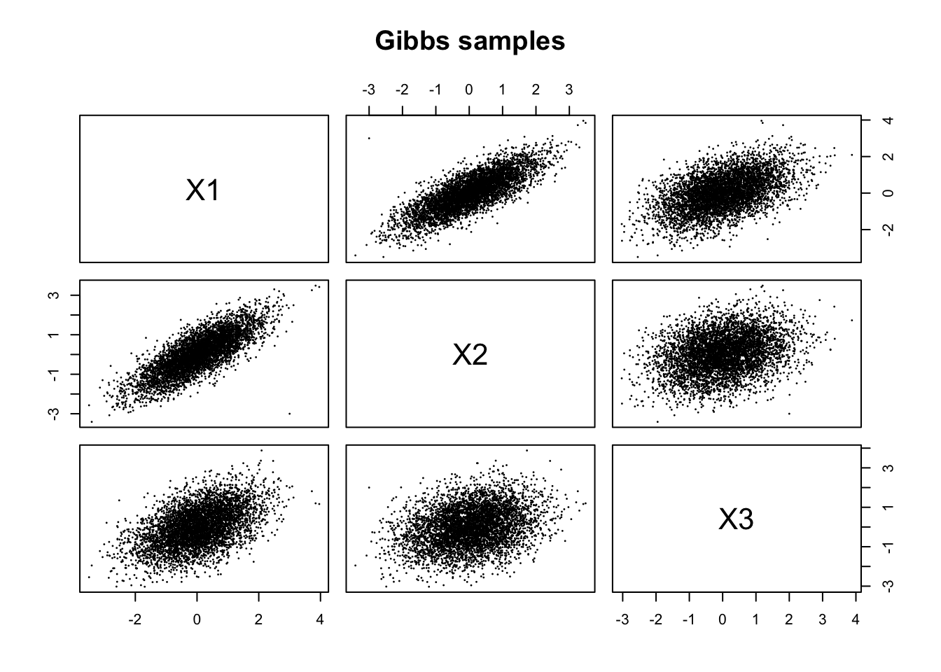

import numpy as np
import matplotlib.pyplot as plt
import pandas as pd

np.random.seed(1234)

# Target covariance matrix
Sigma = np.array([
    [1,   0.8, 0.5],
    [0.8, 1,   0.3],
    [0.5, 0.3, 1]
])

mu = np.array([0, 0, 0])

# Function for conditional normal parameters
def cond_params(j, x, mu, Sigma):
    
    # Indices of other variables
    other = [k for k in range(len(x)) if k != j]
    
    # Extract relevant submatrices and vectors
    Sigma_j_other = Sigma[j, other]
    Sigma_other_other = Sigma[np.ix_(other, other)]
    Sigma_other_j = Sigma[other, j]
    
    mu_j = mu[j]
    mu_other = mu[other]
    
    # Conditional mean
    cond_mean = (
        mu_j
        + Sigma_j_other
        @ np.linalg.inv(Sigma_other_other)
        @ (x[other] - mu_other)
    )
    
    # Conditional variance
    cond_var = (
        Sigma[j, j]
        - Sigma_j_other
        @ np.linalg.inv(Sigma_other_other)
        @ Sigma_other_j
    )
    
    return {
        "mean": cond_mean,
        "sd": np.sqrt(cond_var)
    }

# Gibbs sampler
n = 5000
x = np.zeros((n, 3))

# Starting value
x[0, :] = np.array([3, -3, 2])

for i in range(1, n):
    
    current = x[i - 1, :].copy()
    
    for j in range(x.shape[1]):
        
        cp = cond_params(j, current, mu, Sigma)
        
        current[j] = np.random.normal(
            loc=cp["mean"],
            scale=cp["sd"]
        )
    
    x[i, :] = current

# Convert to DataFrame for convenience
df = pd.DataFrame(x, columns=["X1", "X2", "X3"])

# Pairwise scatter plots
pd.plotting.scatter_matrix(
    df,
    figsize=(8, 8),
    diagonal='hist'
)

plt.suptitle("Gibbs Samples")
plt.show()

The pairwise plots show elliptical point clouds. The strongest relationship appear between \(X_1\) and \(X_2\), since their covariance is 0.8. The relationship between \(X_1\) and \(X_3\) is also positive but weaker, while the relationship between \(X_2\) and \(X_3\) is the weakest of the three.

Trace Plots

A trace plot displays the sampled values over iteration number. Trace plots help assess convergence, mixing behaviour, and stability of the chain.

Good trace plots:

• fluctuate around a stable region;
• show no obvious trend;
• explore the distribution well.

Poor trace plots may indicate:

• slow convergence;
• poor mixing;
• strong autocorrelation.

From Example 2, we can plot the trace of each variable across iterations:

par(mfrow = c(3, 1), mar = c(2, 4, 1, 1))
plot(x[, 1], type = "l", ylab = "X1")
plot(x[, 2], type = "l", ylab = "X2")
plot(x[, 3], type = "l", ylab = "X3")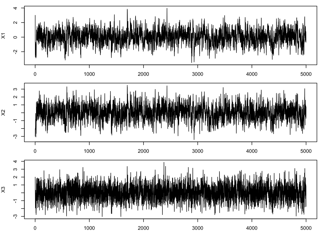

fig, axes = plt.subplots(3, 1, figsize=(10, 8), sharex=True)
axes[0].plot(x[:, 0], color='blue')
axes[0].set_ylabel("X1")
axes[1].plot(x[:, 1], color='green')
axes[1].set_ylabel("X2")
axes[2].plot(x[:, 2], color='red')
axes[2].set_xlabel("Iteration")
axes[2].set_ylabel("X3")
plt.suptitle("Trace Plots for Gibbs Samples")
plt.show() 

The trace plots show that the samples fluctuate around stable regions, with no obvious trends. However, the samples appear to be highly autocorrelated, especially for \(X_1\) and \(X_2\). This is a common feature of Gibbs sampling, since each update depends on the previous state of the chain.

Burn-in Period

The early part of the chain may depend heavily on the starting values. This initial transient behaviour is called the burn-in period. Typically, early samples are discarded, and only later samples are used for inference. The idea is that the chain needs time to approach the target distribution.

The burn-in period is often assessed using trace plots. If the Markov chain appears to have moved away from its initial values and fluctuates around a stable region, the early iterations may be discarded as burn-in. In practice, a common choice is to discard the first 1000 iterations, although the appropriate burn-in length depends on the specific problem, starting values, and convergence behaviour of the chain.

Caution

Burn-in selection is partly subjective, and more formal convergence diagnostics are often used in advanced applications.

From Example 2, we can discard the first 1000 iterations and plot the post-burn-in samples:

burnin <- 1000
x_post <- x[(burnin + 1):n, ]
pairs(x_post, pch = 16, cex = 0.3, 
      main = "Gibbs samples after burn-in")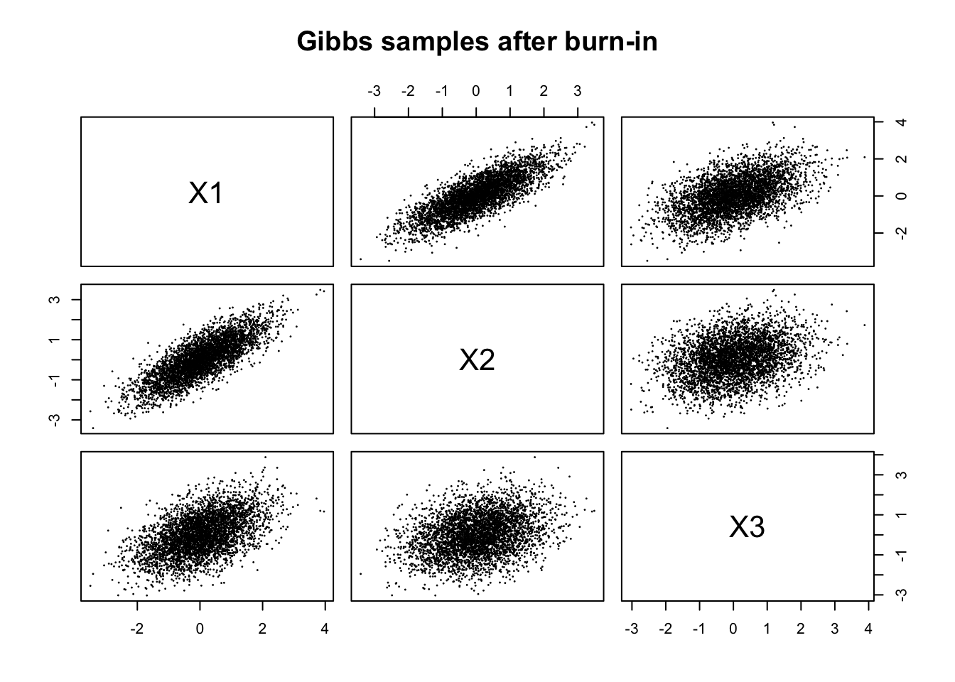

burnin = 1000
x_post = x[burnin:, :]
df_post = pd.DataFrame(x_post, columns=["X1", "X2", "X3"])
pd.plotting.scatter_matrix(
    df_post,
    figsize=(8, 8),
    diagonal='hist'
)
plt.suptitle("Gibbs Samples after Burn-in")
plt.show()

The post-burn-in samples still show the same elliptical relationships as before, but the initial transient behaviour has been removed. It might not look clearly different in this case, but in other examples, the burn-in period can have a significant impact on the quality of the samples and the resulting inference.

Autocorrelation in MCMC

Unlike ordinary Monte Carlo simulation, Gibbs samples are dependent. Successive samples are often highly correlated. This dependence is measured by autocorrelation.

Strong autocorrelation means:

• the chain moves slowly;
• fewer effectively independent samples are obtained.

This is one reason MCMC methods may require many iterations.

The dependence structure connects naturally to ideas from Time Series Modelling. From Example 2, we can plot the autocorrelation function (ACF) for each variable:

par(mfrow = c(3, 1), mar = c(1, 4, 1, 1))
acf(x_post[, 1], ylab = "ACF: X1")
acf(x_post[, 2], ylab = "ACF: X2")
acf(x_post[, 3], ylab = "ACF: X3")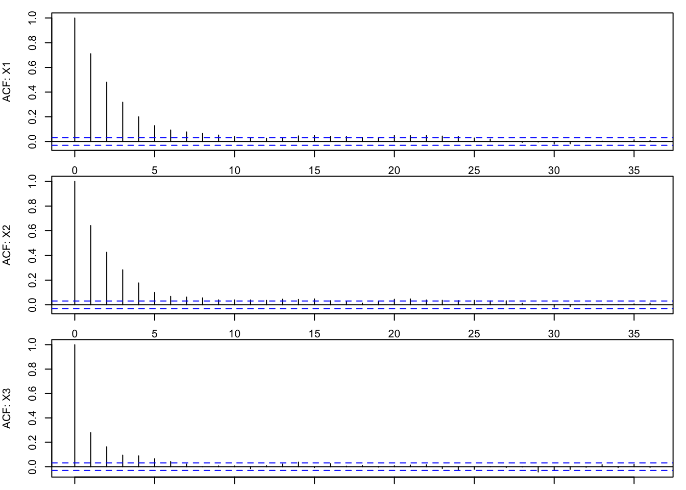

The ACF plots show strong autocorrelation for all three variables, especially at low lags. This indicates that the samples are highly dependent, which is a common feature of Gibbs sampling.

---

Strengths and Limitations

Gibbs sampling has several important strengths.

1. Easy conditional updates If conditional distributions are known and easy to sample from, implementation is straightforward.
2. Effective for high-dimensional models Gibbs sampling is widely used in:
   • Bayesian statistics;
   • hierarchical models;
   • machine learning;
   • image analysis.
3. Avoids difficult normalising constants The full joint density only needs to be known up to proportionality. This is crucial in Bayesian inference.

Despite its usefulness, Gibbs sampling also has limitations.

1. Conditional distributions must be tractable: Sampling from the conditional distributions must be feasible.

2. Slow mixing: Strong dependence between variables may cause slow exploration of the target distribution.

3. Correlated samples: MCMC samples are dependent, reducing statistical efficiency.

Gibbs Sampling in Bayesian Statistics

One of the most important applications of Gibbs sampling is Bayesian inference.

In Bayesian models:

• posterior distributions are often analytically intractable;
• conditional posterior distributions are frequently available in closed form.

The Gibbs sampler allows:

• sequential updating of parameters;
• approximation of posterior means, variances, and intervals;
• full uncertainty quantification.

This transformed Bayesian statistics from a largely theoretical field into a practical computational framework.

The key idea is:

repeatedly sample each parameter from its full conditional posterior distribution given the current values of all other parameters.

General Bayesian Gibbs Sampling Framework

Suppose a Bayesian model has parameters \[ \theta = (\theta_1, \theta_2, \dots, \theta_d) \]

and observed data \(y\). The posterior distribution is

\[ p(\theta \mid y) \propto p(y \mid \theta) p(\theta), \]

where \(p(y \mid \theta)\) is the likelihood and \(p(\theta)\) is the prior. The Gibbs sampler generates samples from the posterior by iteratively sampling each parameter from its full conditional distribution:

\[ \theta_i^{(t+1)} \sim p(\theta_i \mid \theta_{-i}^{(t)}, y), \quad i = 1, \dots, d, \]

where \(\theta_{-i}\) denotes all parameters except \(\theta_i\).

Algorithmic Steps for Bayesian Gibbs Sampling

Step 0 — Derive conditional posteriors

Recall from Statistical Inference chapter, the posterior distribution is proportional to the product of the likelihood and the prior. Therefore, we have to

1. write down the likelihood function \(p(y \mid \theta)\);
2. specify the prior distribution \(p(\theta)\);
3. derive the full conditional posterior distributions \(p(\theta_i \mid \theta_{-i}, y)\) for each parameter \(\theta_i\) using Bayes’ theorem.

The choice of likelihood and prior is crucial, as it determines the form of the conditional posteriors and the feasibility of Gibbs sampling. Usually, conjugate priors are chosen to ensure that the conditional posteriors have standard forms that can be sampled from directly.

Bayesian normal model and Bayesian linear regression are two common examples where conjugate priors lead to tractable conditional posteriors. See the next section for more details.

Step 1 — Choose starting values

\[ \theta_1^{(0)}, \theta_2^{(0)}, \dots, \theta_d^{(0)}. \]

Step 2 — Sequential conditional updates

For iteration \(t = 0,1,2,\cdots,\) update each parameter sequentially

\[ \theta_1^{(t+1)} \sim p(\theta_1 \mid \theta_2^{(t)}, \dots, \theta_d^{(t)}, y), \] \[ \theta_2^{(t+1)} \sim p(\theta_2 \mid \theta_1^{(t+1)}, \theta_3^{(t)}, \dots, \theta_d^{(t)}, y), \] \[ \vdots \] \[ \theta_d^{(t+1)} \sim p(\theta_d \mid \theta_1^{(t+1)}, \dots, \theta_{d-1}^{(t+1)}, y). \]

Step 3 — Repeat

Repeat for many iterations. The generated sequence approximates samples from the posterior distribution.

Example Structured Bayesian Model

• For a Baysian normal model, we have \[ y_i \sim N(\mu, \sigma^2), \qquad i=1,2,\dots,n, \] where \(y_i\) are the observed data, \(\mu\) is the unknown mean parameter, and \(\sigma^2\) is the unknown variance parameter. The following table summarises the conditional posterior distributions for \(\mu\) and \(\sigma^2\):

Parameter	Conditional Posterior
\(\mu\)	Normal
\(\sigma^2\)	Inverse-Gamma

• For a Bayesian linear regression model, we have \[ y = X\beta + \epsilon, \qquad\epsilon \sim N(0, \sigma^2 I), \] where \(y\) is the response vector, \(X\) is the design matrix, \(\beta\) is the vector of regression coefficients, and \(\sigma^2\) is the error variance.

Parameter	Conditional Posterior
\(\beta\)	Multivariate Normal
\(\sigma^2\)	Inverse-Gamma

There are many other examples of structured Bayesian models, such as hierarchical models, mixture models, and time series models, where Gibbs sampling can be applied to perform inference. However, this is beyond the scope of this unit.

43.2 Metropolis-Hastings

Gibbs sampling works well when conditional distributions can be sampled directly. However, this is not always possible.

In more complicated settings:

• conditional distributions may not have standard forms;
• direct conditional sampling may be difficult.

This motivates more general MCMC methods such as Metropolis–Hastings algorithms. Metropolis–Hastings is a general MCMC algorithm that can be used when direct sampling from the conditional distributions is not feasible. The key idea is to propose new samples from a proposal distribution and then accept or reject them based on an acceptance probability that ensures the Markov chain has the correct stationary distribution.

The Metropolis–Hastings algorithm can draw samples from any probability distribution with probability density \(P(x)\), provided that we know a function \(f(x)\) proportional to the density \(P(x)\) and the values of \(f(x)\) can be calculated. The requirement of knowing \(f(x)\) is crucial, as it allows us to compute the acceptance probability without needing to know the normalising constant of the target distribution.

Metropolis–Hastings Algorithm

Let \(f(x)\) be a function that is proportional to the target distribution \(\pi(x)\) we want to sample from:

Step 1 — Initialisation

Start with an initial state \(X^{(0)}\) at \(t=0.\)

Step 2 — Iteration

For each iteration \(t = 1, 2, \ldots, N\):

1. Proposal: At iteration \(t,\) generate a new state \(X^*\) from a proposal distribution \(q(X^* | X^{(t)})\).

2. Acceptance Probability: Calculate the acceptance probability \(\alpha\): \[ \alpha = \min\left(1, \frac{\pi(X^*)\,q(X^{(t)} | X^*)}{\pi(X^{(t)})\,q(X^* | X^{(t)})}\right). \]

3. Accept or Reject:

   • Generate a uniform random number \(u \sim \text{Uniform}(0,1)\).
   • If \(u \leq \alpha\), accept the proposed state and set \(X^{(t+1)} = X^*\).
   • Otherwise, reject the proposed state and set \(X^{(t+1)} = X^{(t)}\).

4. Repeat: Repeat steps 1 to 3 for the desired number of iterations \(N\).

NoteAcceptance Probability (Intuition)

Suppose that the most recent state of the Markov chain is \(X^{(t)}\). The Metropolis–Hastings algorithm proposes a new state \(X^*\) from the proposal distribution \(q(X^* | X^{(t)})\) with the acceptance probability \(\alpha = \min\left(1, a\right)\), where

\[ a = a_1 \cdot a_2 = \frac{\pi(X^*)}{\pi(X^{(t)})} \cdot \frac{q(X^{(t)} | X^*)}{q(X^* | X^{(t)})}. \]

If \(a \geq 1, X^{(t+1)} = X^*\). Otherwise,

• \(X^{(t+1)} = X^*\) with probability \(a\) and
• \(X^{(t+1)} = X^{(t)}\) with probability \(1-a\).

Here,

• \(a_1\) is the probability ratio between the proposed state \(X^*\) and the current state \(X^{(t)}\). This ratio indicates how much more likely the proposed state is compared to the current state under the target distribution.

• \(a_2\) is the ratio of the proposal distributions in two directions (from current to proposed and conversely), which accounts for the asymmetry in the proposal mechanism. If the proposal distribution is symmetric, \(a_2 = 1\).

• The acceptance probability \(\alpha\) is the minimum of 1 and \(a\). This means that if the proposed state is more likely than the current state (i.e., \(a \geq 1\)), it will always be accepted. If the proposed state is less likely (i.e., \(a < 1\)), it will be accepted with probability \(a\), allowing for occasional moves to less likely states, which helps the chain explore the entire target distribution.

Example 3: Truncated Normal Distribution

Suppose we want to sample from a target distribution that is proportional to a truncated normal distribution on the interval \([Lb, Ub] = [-4, 4]\). We can use an independence Metropolis–Hastings algorithm with a uniform proposal distribution over the same interval. The proposal distribution does not depend on the current state, which simplifies the acceptance probability.

set.seed(1234)

# Bounds of uniform prior / proposal
Lb <- -4
Ub <-  4

# Target posterior: proportional to Normal(0, 1), truncated to [Lb, Ub]
posterior <- function(theta) {
  ifelse(theta >= Lb & theta <= Ub, 
         dnorm(theta, mean = 0, sd = 1), 0)
}

# Independence Metropolis-Hastings with proposal q(theta*) = Uniform(Lb, Ub)
N <- 5000
theta <- numeric(N)
accepted <- logical(N)

# Initial value
theta[1] <- runif(1, Lb, Ub)

for (t in 2:N) {
  # Propose a new state from the uniform proposal distribution
  proposal <- runif(1, Lb, Ub)
  
  # Acceptance probability simplifies to ratio of posteriors since proposal is symmetric
  alpha <- min(1, posterior(proposal) / posterior(theta[t - 1]))
  
  # Accept or reject the proposal
  if (runif(1) < alpha) {
    theta[t] <- proposal
    accepted[t] <- TRUE
  } else {
    theta[t] <- theta[t - 1]
    accepted[t] <- FALSE
  }
}

par(mfrow = c(2, 1), mar = c(4, 4, 2, 1))
plot(theta, type = "l", ylab = expression(theta), xlab = "MH iteration",
     main = "Metropolis-Hastings Sampling Path")
hist(theta[(1000 + 1):N], breaks = 30, freq = FALSE, 
     main = "Target Distribution", xlab = expression(theta), ylab = "Density")
curve(posterior(x), add = TRUE, col = "red", lwd = 2)
legend("topright", legend = c("MCMC samples", "True density"),
       col = c("grey", "red"), lwd = c(5, 2), bty = "n")

import numpy as np
import matplotlib.pyplot as plt
np.random.seed(1234)
# Bounds of uniform prior / proposal
Lb = -4
Ub = 4
# Target posterior: proportional to Normal(0, 1), truncated to [Lb, Ub]
def posterior(theta):
    return np.where((theta >= Lb) & (theta <= Ub),
                    np.exp(-0.5 * theta**2) / np.sqrt(2 * np.pi), 0)
# Independence Metropolis-Hastings with proposal q(theta*) = Uniform(Lb, Ub)
N = 5000
theta = np.zeros(N)
accepted = np.zeros(N, dtype=bool)
# Initial value
theta[0] = np.random.uniform(Lb, Ub)
for t in range(1, N):
    # Propose a new state from the uniform proposal distribution
    proposal = np.random.uniform(Lb, Ub)
    # Acceptance probability simplifies to ratio of posteriors since proposal is symmetric
    alpha = min(1, posterior(proposal) / posterior(theta[t - 1]))
    # Accept or reject the proposal
    if np.random.uniform() < alpha:
        theta[t] = proposal
        accepted[t] = True
    else:
        theta[t] = theta[t - 1]
        accepted[t] = False

fig, axes = plt.subplots(2, 1, figsize=(10, 8))
axes[0].plot(theta, color='blue')
axes[0].set_xlabel("MH iteration")
axes[0].set_ylabel("theta")
axes[0].set_title("Metropolis-Hastings Sampling Path")
axes[1].hist(theta[1000:], bins=30, density=True, color='grey', edgecolor='black')
x = np.linspace(Lb, Ub, 500)
axes[1].plot(x, posterior(x), color='red', linewidth=2)
axes[1].set_xlabel("theta")
axes[1].set_ylabel("Density")
axes[1].set_title("Target Distribution")
axes[1].legend(["MCMC samples", "True density"])
plt.tight_layout()
plt.show()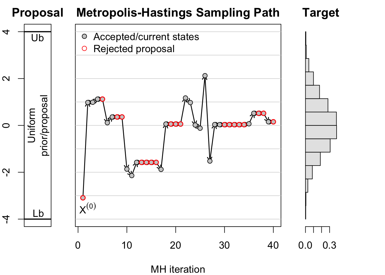

Figure 43.3: Schematic of Metropolis–Hastings Algorithm

The Figure 43.3 illustrates the Metropolis–Hastings algorithm. The left panel shows the proposal distribution, which is uniform over the interval \([Lb, Ub]\). The middle panel shows the sampling path of the Markov chain over the first 40 iterations. Arrows indicate the transitions between states, with red circles marking rejected proposals. The rejection results in a horizontal repetition of the previous state. The right panel shows a histogram of the post-burn-in samples, which approximates the target distribution proportional to a truncated normal.

Comparison: Gibbs vs Metropolis–Hastings

Gibbs sampling is a special case of the Metropolis–Hastings algorithm where proposals are generated directly from the conditional distributions. In this case, the acceptance probability is always 1, so every proposal is accepted.

Feature	Gibbs Sampling	Metropolis–Hastings (MH)
Update mechanism	Sequential conditional updates	Proposal + acceptance probability
Example update	\(X_j^{(t+1)} \sim p(X_j \mid X_{-j},y)\)	Propose \(X^\ast \sim q(X^\ast\mid X^{(t)})\), then accept/reject
Proposal distribution?	No explicit proposal distribution	Yes
Conditional distributions?	Yes	No
Acceptance step & probability?	No (probability always 1)	Yes (probability < 1)
Can remain at same state?	Usually no repeated rejection step	Yes, rejected proposals keep current state
When useful	Conditional distributions have standard forms	Direct conditional sampling is difficult
Typical applications	Bayesian normal models, hierarchical models	General Bayesian inference, complex posteriors
Efficiency	Often efficient for conjugate models	Depends heavily on proposal distribution

---

1. Normal PDF: \(f(x) = \frac{1}{\sqrt{2\pi\sigma^2}} \exp\left(-\frac{(x-\mu)^2}{2\sigma^2}\right)\)

2. marginal variance for both \(X\) and \(Y\) is 1