3  Workshop Activities

Objectives

This workshop consists of two parts:

• Part 1: Introduction to R and development environments
• Part 2: Probability Foundations for Simulation

By the end of this workshop, you should be able to:

1. Navigate and use R effectively within R Notebook and RStudio;

2. Implement basic R functions relevant to simulation tasks (e.g., variables, functions, loops, and random number generation);

3. Recall and apply key probability concepts that underpin simulation methods.

Part 1: Introduction & review to R

Mini tasks

1. Add your name + student ID to the YAML at the top of this notebook using author tag.
2. To verify that you have a running notebook, run a code cell:

sessionInfo()

R version 4.4.3 (2025-02-28)
Platform: aarch64-apple-darwin20
Running under: macOS 26.3.1

Matrix products: default
BLAS:   /Library/Frameworks/R.framework/Versions/4.4-arm64/Resources/lib/libRblas.0.dylib 
LAPACK: /Library/Frameworks/R.framework/Versions/4.4-arm64/Resources/lib/libRlapack.dylib;  LAPACK version 3.12.0

locale:
[1] C.UTF-8/C.UTF-8/C.UTF-8/C/C.UTF-8/C.UTF-8

time zone: Australia/Perth
tzcode source: internal

attached base packages:
[1] stats     graphics  grDevices utils     datasets  methods   base     

loaded via a namespace (and not attached):
 [1] htmlwidgets_1.6.4 compiler_4.4.3    fastmap_1.2.0     cli_3.6.5        
 [5] tools_4.4.3       htmltools_0.5.9   otel_0.2.0        rmarkdown_2.30   
 [9] knitr_1.51        jsonlite_2.0.0    xfun_0.56         digest_0.6.39    
[13] rlang_1.1.7       evaluate_1.0.5   

This prints R version, platform, attached packages, locale, matrix products / BLAS info.

Running Code Chunks in RStudio

RStudio provides several convenient ways to run code chunks in an R Markdown notebook.

Using the Run Button

• Click the Run button at the top right of a code chunk to execute that chunk.
  
• The output appears immediately below the chunk.

Using Keyboard Shortcuts

• Ctrl + Enter (Windows/Linux) or Cmd + Enter (macOS):
  Runs the current line or selected code and moves the cursor to the next line.
• Ctrl + Shift + Enter (Windows/Linux) or Cmd + Shift + Enter (macOS):
  Runs the entire code chunk.
• Alt + Enter (Windows/Linux) or Option + Enter (macOS):
  Inserts a new code chunk.

Running Multiple Chunks

• Run All Chunks Above:
  Click the small dropdown next to the Run button and choose Run All Chunks Above.
• Run All Chunks Below:
  Same dropdown → Run All Chunks Below.
• Run All:
  Use Run All to execute every chunk in the document sequentially.

Running the Entire Document

• Click Knit to run all chunks and render the document into HTML, PDF, or Word (depending on your YAML settings).

Insert a code Chunk

If you are using R Notebook/Markdown within the RStudio IDE, you can also use a keyboard shortcut or toolbar button to insert a chunk with the necessary R syntax automatically.

• Keyboard Shortcut: Press Ctrl + Alt + I (Windows/Linux) or Cmd + Option + I (macOS).

Learning R with the swirl Package

The swirl package is an interactive learning tool that teaches R programming and data science inside your RStudio console. It guides you through short lessons, checks your answers, and gives immediate feedback — perfect for beginners who want hands‑on practice. In this workshop, you will install swirl, start a lesson, and complete a few interactive exercises.

Why use swirl?

• It teaches R from within R
• Lessons are short, structured, and beginner‑friendly
• You get instant feedback on your answers
• You can learn at your own pace
• It reinforces the skills you’ll use in simulation labs

install.packages("swirl")
library(swirl)
swirl() # begin interactive session

For STAT2005, the following swirl lessons are most relevant:

• R Programming (especially: Basic Building Blocks, Workspace and Files, Sequences, Vectors, Logic, Functions, lapply/sapply)
  
• Data Science: Foundations using R (optional but helpful)

Part 2: Probability Foundations for Simulation

Here is a collection of summary and reference sheets I prepared for STAT1005:

• Summary of Theory
• Probability Distributions Reference Sheet
• Hypothesis Testing Reference Sheet

Random Number Generator

Simulation begins with the ability to generate random‑looking numbers. Computers, however, are deterministic machines—they cannot produce true randomness on their own. Instead, they use pseudorandom number generators (PRNGs): algorithms that produce sequences of numbers that behave like random samples.

In this section, we will:

• implement a simple Linear Congruential Generator (LCG)
• generate Uniform(0,1) samples
• compare our LCG to built‑in generator

This gives us the computational foundation for all later simulation work.

LCGs

From the lecture, we learned that an LCG produces a sequence of integers using a recurrence relation: \[ X_{n+1} = (aX_n + c) \mod m, \] where \(X\) is the sequence of pseudo-random values and

• the modulus \(m, 0 < m\)
• the multiplier \(a, 0 < a < m\)
• the increment \(c, 0 \leq c < m\)
• the seed or start values \(X_0, 0 \leq X_0 < m\)

Good choices of \((a,c,m)\) give long, well‑distributed sequences. Poor choices give visible patterns—great for teaching, not great for real simulation.

Exercise 3.1

3.1.1 Write a function lcg() that produces a sequence of integers using a recurrence relation above. Try different parameter values.

3.1.2 Write a function lcg_uniform() that returns the LCG integer output scaled to Uniform(0,1).

3.1.3 Plot a histogram of lcg_uniform(10_000)

3.1.4 Plot a histogram of the built in Uniform generator runif()

Probability Distributions (PDF/PMF/CDF)

Discrete RVs (e.g., Bernoulli, Binomial) PMF gives the probability of each possible value \[ P(X=x) \] Continuous RVs (e.g., Exponential, Normal) - PDF describes the shape of the distribution \[ f(x) \] - CDF gives cumulative probability \[ F(x)=P(X\leq x) \] Simulation gives us samples. Theory gives us functions.

Example: Exponential(λ)

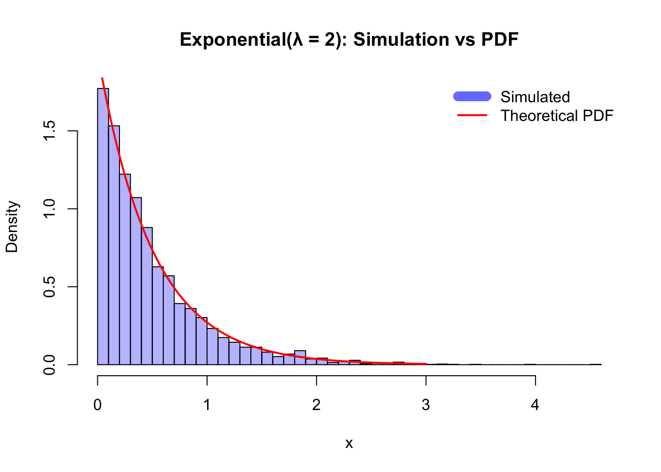
We already simulated Exponential(λ) using inverse transform. Now we compare the simulated histogram to the theoretical PDF: \[ f(x)=\lambda e^{-\lambda x},\quad x\geq 0 \]

# Simulate
lam <- 2
samples <- -log(runif(5000)) / lam

# Theoretical PDF
x <- seq(0, 3, length.out = 300)
pdf <- lam * exp(-lam * x)

# Plot
hist(samples,
     breaks = 40,
     freq = FALSE,
     col = rgb(0, 0, 1, 0.3),
     border = "black",
     main = "Exponential(λ = 2): Simulation vs PDF",
     xlab = "x")

lines(x, pdf, col = "red", lwd = 2)
legend("topright",
       legend = c("Simulated", "Theoretical PDF"),
       col = c(rgb(0, 0, 1, 0.6), "red"),
       lwd = c(10, 2),
       bty = "n")

Exercise 3.2

The Normal distribution has PDF: \[ f(x)=\frac{1}{\sqrt{2\pi }}e^{-x^2/2} \] Use rnorm() to simulate Normal(0, 1) data and dnorm() to compute the theoretical PDF, then create a comparison plot similar to the example above.

Example: Bernoulli(p)

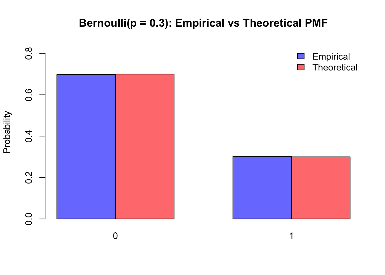
For Bernoulli(p), the theoretical PMF: \[ P(X=1)=p,\quad P(X=0)=1-p \]

# Parameter
p <- 0.3

# Simulate Bernoulli samples
samples_bern <- as.integer(runif(5000) < p)

# Empirical PMF
counts <- table(samples_bern)
empirical <- counts / sum(counts)

# Theoretical PMF
theoretical <- c("0" = 1 - p, "1" = p)

# Plot
barplot(
  rbind(empirical, theoretical),
  beside = TRUE,
  col = c(rgb(0, 0, 1, 0.6), rgb(1, 0, 0, 0.6)),
  names.arg = c("0", "1"),
  ylim = c(0, max(empirical, theoretical) * 1.2),
  main = "Bernoulli(p = 0.3): Empirical vs Theoretical PMF",
  ylab = "Probability"
)

legend(
  "topright",
  legend = c("Empirical", "Theoretical"),
  fill = c(rgb(0, 0, 1, 0.6), rgb(1, 0, 0, 0.6)),
  bty = "n"
)

Law of Large Numbers (LLNs)

The Law of Large Numbers (LLN) is one of the most important ideas in probability and simulation. It explains why simulation works and why empirical averages converge to theoretical expectations. In simple terms:

As we take more and more samples, the sample mean gets closer to the true mean.

This is why Monte Carlo methods are powerful: averages stabilise. We’ll demonstrate LLN using simulation.

LLNs with Binomial

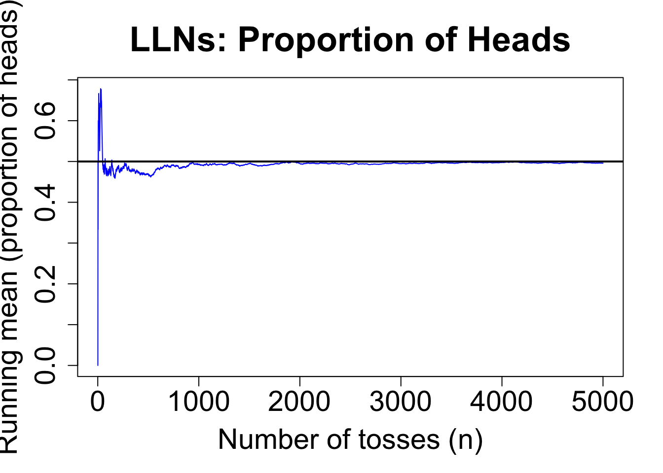
Consider coin tosses example,

set.seed(123)
n <- 5000

x <- rbinom(5000, size = 1, prob = 0.5)   # 1 = Head, 0 = Tail
running_mean <- cumsum(x) / seq_len(n)

plot(running_mean, type = "l", col = "blue",
     xlab = "Number of tosses (n)",
     ylab = "Running mean (proportion of heads)",
     main = "LLNs: Proportion of Heads",
     cex.main = 2.2,
     cex.lab = 1.8,
     cex.axis = 1.8,
     )

abline(h = 0.5, lwd = 2)  # true mean

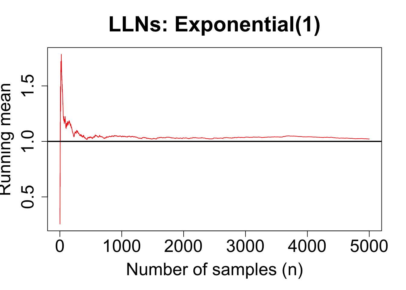
LLNs with Exp(1)

set.seed(2026)
x <- rexp(n, rate = 1)
running_mean <- cumsum(x) / seq_len(n)

plot(running_mean, type = "l", col = "red",
     xlab = "Number of samples (n)",
     ylab = "Running mean",
     main = "LLNs: Exponential(1)",
      cex.main = 2.2,
     cex.lab = 1.8,
     cex.axis = 1.8,
     )

abline(h = 1, lwd = 2)  # true mean

Exercise 3.3

For a Uniform(0,1) random variable with \(\mathbb{E}[X]=0.5\), use runif() to simulate 5000 samples and create a plot to demonstrate the LLNs.