set.seed(1234)
n <- 1000
white_noise <- rnorm(n, mean = 0, sd = 1)
plot(white_noise, type = "l", main = "Gaussian White Noise Process", xlab = "Time", ylab = "Value")
abline(h = 0, col = "red", lty = 2)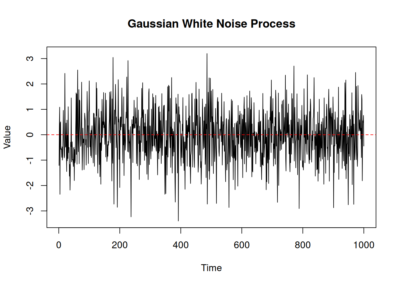
We begin the study of time series modelling with the simplest stochastic process with no temporal dependence: white noise. White noise represents a sequence of random variables that exhibit no temporal structure, serving as a fundamental benchmark against which all dependent processes are compared.
Formally, white noise is a stochastic process indexed by time, denoted as \[ \{ \varepsilon_t : t = 1, 2, \dots \}, \quad \varepsilon_t \sim \text{i.i.d. } (0, \sigma^2) \]
where \(\varepsilon_t\) represents the value of the process at time \(t\), and \(\sigma^2\) is the variance. It is characterised by the following properties:
\[ \mathbb{E}(\varepsilon_t) = 0, \quad \text{Var}(\varepsilon_t) = \sigma^2, \quad \text{Cov}(\varepsilon_t, \varepsilon_s) = 0 \text{ for } t \neq s \]
Independence implies that observations at different times carry no information about one another, while identical distribution ensures that the variability and distributional shape remain the same at every time point.
From a simulation perspective, white noise corresponds to repeatedly generating independent random draws from a fixed distribution. When visualised as a time series, a white noise process fluctuates randomly around its mean, displaying no persistence, trend, or systematic pattern. Large values are just as likely to be followed by small values as by large ones; positive and negative fluctuations occur without memory of the past.
White noise can be generated from any distribution (normal, uniform, t-distribution, discrete, etc.), but the most common case is Gaussian white noise, where each \(\varepsilon_t\) is drawn from a normal distribution with mean zero and variance \(\sigma^2\). This choice is often made for mathematical convenience and because many aggregated random effects tend to produce approximately Gaussian behaviour.
Example: Simulate Gaussian white noise process with mean zero and variance one:
\[ \varepsilon_t \sim \text{i.i.d. } N(0, 1) \]
set.seed(1234)
n <- 1000
white_noise <- rnorm(n, mean = 0, sd = 1)
plot(white_noise, type = "l", main = "Gaussian White Noise Process", xlab = "Time", ylab = "Value")
abline(h = 0, col = "red", lty = 2)
import numpy as np
import matplotlib.pyplot as plt
np.random.seed(1234)
n = 1000
white_noise = np.random.normal(loc=0, scale=1, size=n)
plt.plot(white_noise, color='blue')
plt.axhline(0, color='red', linestyle='--')
plt.title('Gaussian White Noise Process')
plt.xlabel('Time')
plt.ylabel('Value')
plt.show()
The above code simulates a Gaussian white noise process with 1000 observations drawn from a standard normal distribution. The resulting plot shows
consistent with the properties of white noise.
Even in pure white noise, the human eye may perceive short runs or apparent patterns. These are artefacts of randomness rather than evidence of structure.
The defining characteristic of white noise is the absence of memory. Knowing the current or past values of the process provides no information about future outcomes. This makes white noise fundamentally different from many real-world systems, where past states influence future behaviour. Formally, we can express this lack of dependence as:
In this sense, white noise plays a role analogous to independence in random variables: it represents the baseline case against which dependence can be identified and measured. Any observed structure in a time series — such as persistence, cycles, or predictability — must arise from deviations away from white noise behaviour.
This absence of dependence can also be quantified. In particular, we will later see that the autocorrelation function (ACF) of a white noise process is zero at all non-zero lags, reflecting the lack of relationship between observations across time.
Simulating white noise allows us to develop an intuitive understanding of pure randomness in time. By generating multiple sample paths, we can observe the inherent variability of the process and distinguish random fluctuations from genuine temporal structure. Apparent clusters or short runs may occasionally appear, but these do not persist systematically and disappear when viewed across repeated simulations.
Because white noise lacks dependence, it cannot produce meaningful forecasts beyond its mean. Any attempt to predict future values using past observations will perform no better than random guessing. For this reason, white noise often serves as a null model in time series analysis: before introducing more complex dynamics, it is essential to understand what behaviour arises in their absence.
Although white noise is rarely an adequate model for real data, it plays a crucial conceptual role in time series modelling. Many dependent processes are constructed by adding structure to white noise, using it as a source of randomness that drives dynamic systems. In later sections, we will see how simple recursive mechanisms transform white noise into processes with memory, persistence, and meaningful temporal patterns.
Understanding white noise is therefore a prerequisite for understanding time series models. By clearly establishing what “no structure” looks like, we set the foundation for recognising, interpreting, and simulating dependence in time‑evolving systems.