lcg <- function(n, seed, a, c, m) { # this function has 5 arguments
  x <- numeric(n)  # initialise x as numeric vector of size n
  x[1] <- seed     # the first value is X_0 (seed)
  for (i in 2:n) { # recurrent relation calculation in a loop
    x[i] <- (a * x[i - 1] + c) %% m # %%: modulus
  }
  return(x)        # don't forget to return a value!
}4 R Workshop Solutions
Part 2: Probability Foundations for Simulation
Random Number Generator
Simulation begins with the ability to generate random‑looking numbers. Computers, however, are deterministic machines—they cannot produce true randomness on their own. Instead, they use pseudorandom number generators (PRNGs): algorithms that produce sequences of numbers that behave like random samples.
In this section, we will:
- implement a simple Linear Congruential Generator (LCG)
- generate Uniform(0,1) samples
- compare our LCG to built‑in generator
This gives us the computational foundation for all later simulation work.
LCGs
From the lecture, we learned that an LCG produces a sequence of integers using a recurrence relation: \[ X_{n+1} = (aX_n + c) \mod m, \] where \(X\) is the sequence of pseudo-random values and
- the modulus \(m, 0 < m\)
- the multiplier \(a, 0 < a < m\)
- the increment \(c, 0 \leq c < m\)
- the seed or start values \(X_0, 0 \leq X_0 < m\)
Good choices of \((a,c,m)\) give long, well‑distributed sequences. Poor choices give visible patterns, which is not great for real simulation.
Exercise 3.1.1
Write a function lcg() that produces a sequence of integers using a recurrence relation above. Try different parameter values.
In R, you can write a function with or without default arguments. If you don’t give an argument a default value (e.g. seed = 1, a = 5, c = 1, m = 16), you must specify it when you call the function.
- The Numerical Recipes parameters (from the lecture)
set.seed(123)      # for reproducibility: only once per notebook
u <- lcg(n=10000, seed=1, a=1664525, c=1013904223, m=2^32) # simulate
head(u, n=10)      # returns the fist parts of a vector
[1] 1 1015568748 1586005467 2165703038 3027450565 217083232
[7] 1587069247 3327581586 2388811721 70837908Let’s try some other parameters…
You can look up some interesting parameters combinations from LCG: parameters in common use. For example,
- The ZX81, ZX Spectrum parameters
u <- lcg(n=10000, seed=1, a=75, c=0, m=2^16+1)
head(u, n=20)
[1] 1 75 5625 28653 51791 17642 12410 13232 9345 45505 4951 43640
[13] 61687 38935 36497 50258 33741 40169 63510 44586- The Borland C/C++ parameters
u <- lcg(n=10000, seed=1, a=22695477, c=0, m=2^31)
head(u, n=20)
[1] 1 22695477 2133350137 711188368 1567303888 650040080
[7] 1836094032 889367184 1344614352 191120912 448487760 647071120
[13] 1467123408 887703824 1211039824 804483216 1012018640 1914231824
[19] 533884752 647719824We need to scale these integer to Uniform(0,1).
Exercise 3.1.2
Write a function lcg_uniform() that returns the LCG integer output scaled to Uniform(0,1).
# as.uniform = TRUE controls the output of the LCG.
lcg_uniform <- function(n, seed, a, c, m, as.uniform = TRUE) {
  x <- numeric(n)
  x[1] <- seed
  for (i in 2:n) {
    x[i] <- (a * x[i - 1] + c) %% m
  }
  if (as.uniform) {
    return(x / m)   # convert to Uniform(0,1)
  } else {
    return(x)       # return raw integers
  }
}- The Numerical Recipes parameters
u_NR <- lcg_uniform(n=10000, seed=1, a=1664525, c=1013904223, m=2^32)
head(u_NR, 20)
[1] 2.328306e-10 2.364555e-01 3.692707e-01 5.042420e-01 7.048833e-01
[6] 5.054363e-02 3.695184e-01 7.747630e-01 5.561886e-01 1.649324e-02
[11] 6.392460e-01 2.504511e-01 4.223778e-01 5.906902e-01 8.369337e-01
[16] 2.350759e-01 9.808460e-01 8.608871e-01 3.268755e-01 6.826027e-01- The ZX81, ZX Spectrum parameters
ZX Spectrum / ZX81 LCG is another classic historical example. It was/is used for applications like simple games, shuffling sprites, basic procedural effects, etc.
u_ZX <- lcg_uniform(n=10000, seed=1, a=75, c=0, m=2^16+1)
head(u_ZX, 20)
[1] 1.525856e-05 1.144392e-03 8.582938e-02 4.372034e-01 7.902559e-01
[6] 2.691914e-01 1.893587e-01 2.019012e-01 1.425912e-01 6.943406e-01
[11] 7.554511e-02 6.658834e-01 9.412546e-01 5.940919e-01 5.568915e-01
[16] 7.668645e-01 5.148389e-01 6.129209e-01 9.690709e-01 6.803180e-01- The Borland C/C++ parameters
Borland C/C++ is also another classic historical LCG that was good enough for simple simulations, games, non-critical numerical work, etc.
u_BL <- lcg_uniform(n=10000, seed=1, a=22695477, c=0, m=2^31)
head(u_BL, n=20) # also needs diagnostic plots to figure out the quality
[1] 4.656613e-10 1.056841e-02 9.934186e-01 3.311729e-01 7.298327e-01
[6] 3.026985e-01 8.549979e-01 4.141439e-01 6.261349e-01 8.899761e-02
[11] 2.088434e-01 3.013160e-01 6.831826e-01 4.133693e-01 5.639344e-01
[16] 3.746167e-01 4.712579e-01 8.913837e-01 2.486095e-01 3.016180e-01We need diagnostic plots to assess the quality of the parameters used.
Exercise 3.1.3-3.1.4
Plot a diagnostic plots of lcg_uniform(10_000)
par(mfrow = c(1, 2),      # control multi-figure structure (nrows, ncols)
    mar = c(4, 4, 2, 1),  # bottom, left, top, right plot margins
    oma = c(0, 0, 3, 0))  # outer margins (whole figure)
hist(u_NR, breaks=30, col="skyblue", main="", xlab="Value")
# breaks control the breakpoints between histogram cells
plot(u_NR[-length(u_NR)], u_NR[-1], pch=16, cex=0.25)
# use [-length(u_NR)] for location of x to avoid confusion
# [-1] = all elements except the first one
# it's a standard trick to shift the vector by 1
mtext("Diagnostic plots for Numerical Recipes LCG parameters",
      side = 3, outer = TRUE, cex = 1.25) # big title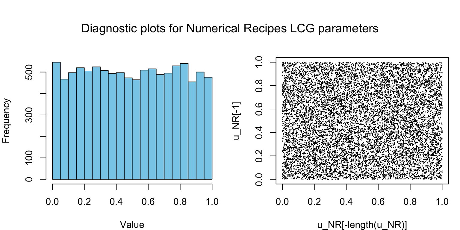
With these parameters, the generator has a maximal period of \(2^{32}\), meaning it cycles through all possible 32‑bit states before repeating (assuming a non‑degenerate seed). So, the NR parameters still produce lattice structure when plotting successive pairs on higher-dimensional tuples. That’s why the NR LCG performs poorly on several modern statistical test suites compared with newer generators. Modern generators (e.g. Mersenne Twister) are vastly superior.
par(mfrow = c(1, 2),
    mar = c(4, 4, 2, 1),
    oma = c(0, 0, 3, 0))
hist(u_ZX, breaks=30, col="skyblue", main="", xlab="Value")
plot(u_ZX[-length(u_ZX)], u_ZX[-1], pch=16, cex=0.25)
mtext("Diagnostic plots for ZX81 / ZX Spectrum parameters",
      side = 3, outer = TRUE, cex = 1.25)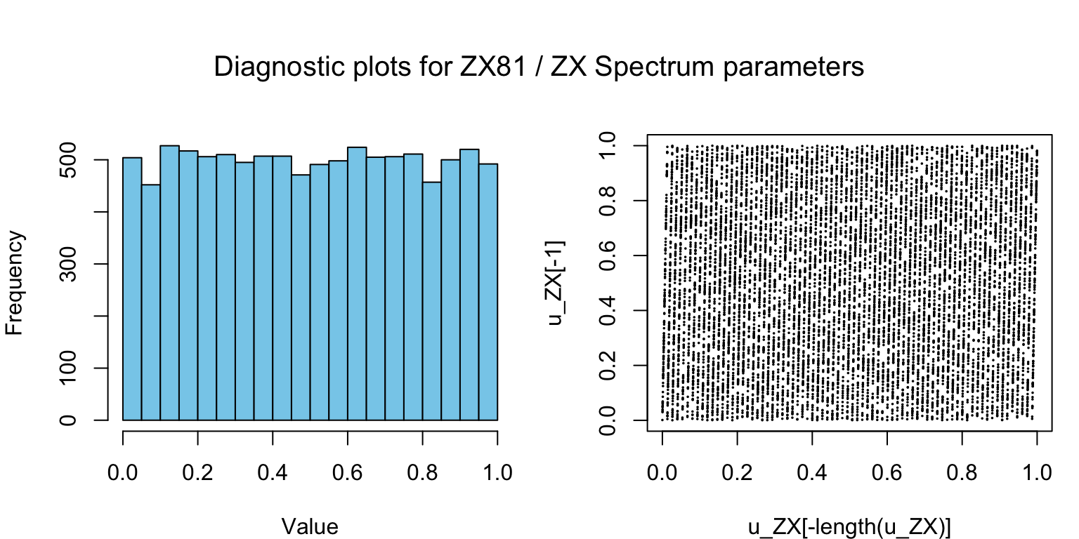
The ZX Spectrum LCG parameters were appropriate for early 8‑bit hardware due to their simplicity and speed, but they exhibit severe statistical weaknesses, including strong lattice structure and poor high‑dimensional behaviour. While adequate for simple games and demonstrations, they are unsuitable for modern simulation and are mainly of pedagogical value today.
par(mfrow = c(1, 2),
    mar = c(4, 4, 2, 1),
    oma = c(0, 0, 3, 0))
hist(u_BL, breaks=30, col="skyblue", main="", xlab="Value")
plot(u_BL[-length(u_BL)], u_BL[-1], pch=16, cex=0.25)
mtext("Diagnostic plots for Berland C/C++  parameters",
      side = 3, outer = TRUE, cex = 1.25)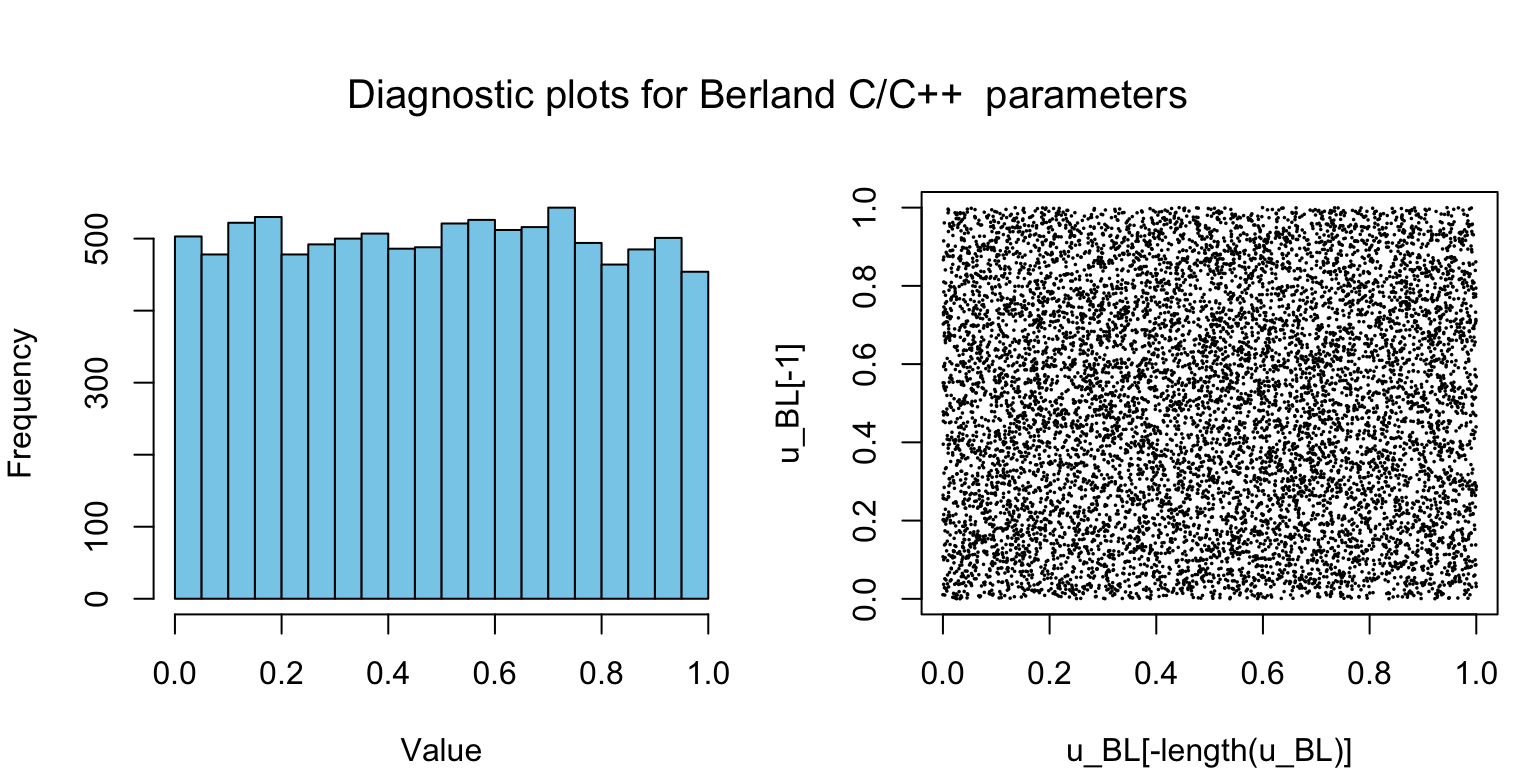
The Borland C/C++ random number generator uses a mixed LCG with a 32‑bit modulus and full period. While it is fast and simple, it suffers from strong lattice structure and poor low‑order bits, making it unsuitable for modern statistical simulation and Monte Carlo methods.
Probability Distributions (PDF/PMF/CDF)
Discrete RVs (e.g., Bernoulli, Binomial): PMF gives the probability of each possible value \[ P(X=x) \] Continuous RVs (e.g., Exponential, Normal): PDF describes the shape of the distribution \[ f(x) \]
CDF gives cumulative probability \[ F(x)=P(X\leq x) \] Simulation gives us samples. Theory gives us functions.
Example: Exponential(λ)
Let’s compare the simulated histogram to the theoretical PDF:
\[ f(x)=\lambda e^{-\lambda x},\quad x\geq 0 \]
# Simulate
lam <- 2
samples <- -log(runif(5000)) / lam    # inverse transform method
# samples <- rexp(5000, rate=lam)     # built-in rexp()

# Theoretical PDF
x <- seq(0, 3, length.out = 300)
pdf <- lam * exp(-lam * x)         # f(x)

# Plot
hist(samples,
     breaks = 40,
     freq = FALSE,
     col = rgb(0, 0, 1, 0.3),
     border = "black",
     main = "Exponential(λ = 2): Simulation vs PDF",
     xlab = "x")

lines(x, pdf, col = "red", lwd = 2)
legend("topright",
       legend = c("Simulated", "Theoretical PDF"),
       col = c(rgb(0, 0, 1, 0.6), "red"),
       lwd = c(10, 2),
bty = "n") VS theoretical PDF of Exp(2)-1.png)
The code uses the inverse transform method to simulate Exponential(λ = 2) random variables, plots their empirical density using a histogram, and overlays the theoretical probability density function for comparison. This highlights the importance of reliable Uniform(0,1) random number generators, such as the Mersenne Twister, which historically enabled simulation from complex distributions before modern built‑in generators were widely available.
You can also try using the built-in rexp() function and compare the histograms.
Exercise 3.2
The Normal distribution has PDF: \[
f(x)=\frac{1}{\sqrt{2\pi }}e^{-x^2/2}
\] Use rnorm() to simulate Normal(0, 1) data and dnorm() to compute the theoretical PDF, then create a comparison plot similar to the example above.
# Simulate Normal(0, 1)
samples <- rnorm(n = 5000, mean = 0, sd = 1)

# Theoretical PDF
x <- seq(-4, 4, length.out = 300)
pdf <- dnorm(x, mean = 0, sd = 1)

# Plot
hist(samples,
     breaks = 40,
     freq = FALSE,
     col = rgb(0, 0, 1, 0.3),
     border = "black",
     main = "Normal(0, 1): Simulation vs PDF",
     xlab = "x")

lines(x, pdf, col = "red", lwd = 2)

legend("topright",
       legend = c("Simulated", "Theoretical PDF"),
       col = c(rgb(0, 0, 1, 0.6), "red"),
       lwd = c(10, 2),
       bty = "n")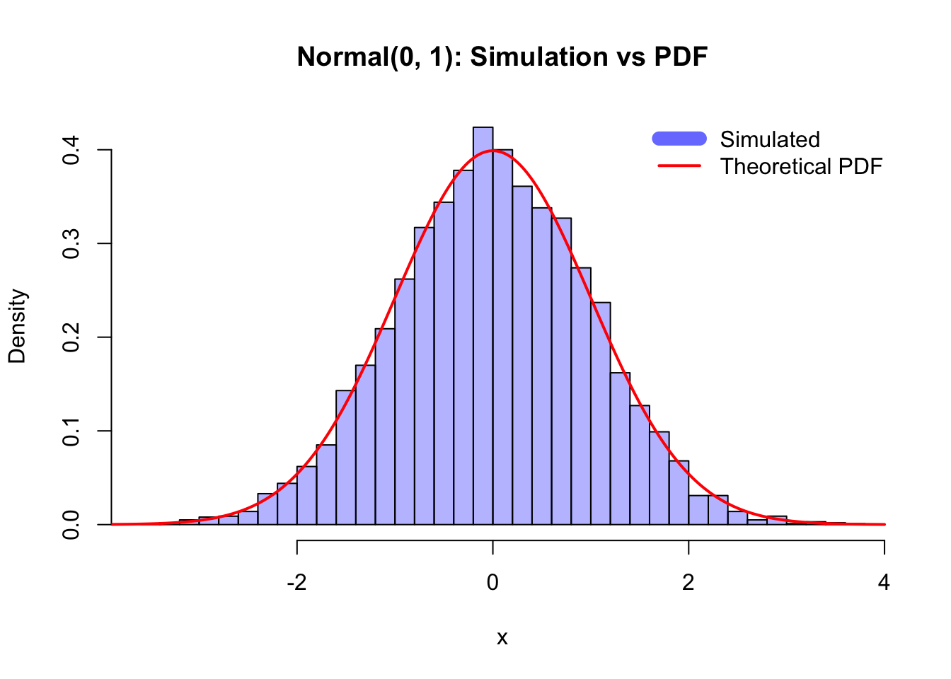
What this is doing (conceptually)
rnorm(5000)generates i.i.d. samples from N(0,1)hist(..., freq = FALSE)scales the histogram to a density, so it’s comparable to a PDFdnorm()computes the exact Normal(0,1) density- The red curve should closely match the histogram as sample size increases
The histogram of simulated Normal(0,1) data approximates the theoretical PDF, and the agreement improves with larger sample sizes due to LLN.
Example: Bernoulli(p)
For Bernoulli(p), the theoretical PMF: \[ P(X=1)=p,\quad P(X=0)=1-p \]
# Parameter
p <- 0.3

# Simulate Bernoulli samples
samples_bern <- as.integer(runif(5000) < p)

# Empirical PMF
counts <- table(samples_bern)
empirical <- counts / sum(counts)

# Theoretical PMF
theoretical <- c("0" = 1 - p, "1" = p)

# Plot
barplot(
  rbind(empirical, theoretical),
  beside = TRUE,
  col = c(rgb(0, 0, 1, 0.6), rgb(1, 0, 0, 0.6)),
  names.arg = c("0", "1"),
  ylim = c(0, max(empirical, theoretical) * 1.2),
  main = "Bernoulli(p = 0.3): Empirical vs Theoretical PMF",
  ylab = "Probability"
)

legend(
  "topright",
  legend = c("Empirical", "Theoretical"),
  fill = c(rgb(0, 0, 1, 0.6), rgb(1, 0, 0, 0.6)),
  bty = "n"
)-1.png)
Law of Large Numbers (LLNs)
The Law of Large Numbers (LLN) is one of the most important ideas in probability and simulation. It explains why simulation works and why empirical averages converge to theoretical expectations. In simple terms:
As we take more and more samples, the sample mean gets closer to the true mean.
This is why Monte Carlo methods are powerful: averages stabilise. We’ll demonstrate LLN using simulation.
Example: LLNs with Binomial
Consider coin tosses example,
n <- 5000
x <- rbinom(n, size = 1, prob = 0.5)   # 1 = Head, 0 = Tail

running_mean <- cumsum(x) / seq_len(n)
# mean = sum of x_i from i->n divided by n
# as n increases, we can calculate running means using the function
# cum_sum(x) : cumulative sums
# seq_len(n) : generate a sequence from 1,2,...,n

plot(running_mean, type = "l", col = "blue",
     xlab = "Number of tosses (n)",
     ylab = "Running mean (proportion of heads)",
     main = "LLNs: Proportion of Heads",
     )
abline(h = 0.5, lwd = 2) # true mean-1.png)
Example: LLNs with Exp(1)
x <- rexp(n, rate = 1)
running_mean <- cumsum(x) / seq_len(n)

plot(running_mean, type = "l", col = "red",
     xlab = "Number of samples (n)",
     ylab = "Running mean",
     main = "LLNs: Exponential(1)",
     )

abline(h = 1, lwd = 2) # true mean-1.png)
Exercise 3.3
For a Uniform(0,1) random variable with \(\mathbb{E}[X]=0.5\), use runif() to simulate 5000 samples and create a plot to demonstrate the LLNs.
# Simulate Uniform(0,1) data
samples <- runif(5000)

# Compute running (cumulative) mean
running_mean <- cumsum(samples) / seq_along(samples)

# Plot the running mean
plot(running_mean,
     type = "l",
     lwd = 2,
     col = "blue",
     ylim = c(0, 1),
     xlab = "Sample size n",
     ylab = "Sample mean",
     main = "LLNs: Uniform(0,1)")

# Add true mean
abline(h = 0.5, col = "red", lwd = 2, lty = 2)

legend("topright",
       legend = c("Running mean", "True mean = 0.5"),
       col = c("blue", "red"),
       lwd = 2,
       lty = c(1, 2),
bty = "n")-1.png)