23 Linear Transformations and the Multivariate Normal

Linear transformations play a central role in probability and statistics, especially when working with multivariate normal distributions. In earlier sections, we saw how a linear transformation of two independent standard normals can create correlation. Here, we generalise that idea and show how any multivariate normal distribution can be constructed from a standard one using a matrix transformation.

Why This Matters

Linear transformations of multivariate normals underpin:

simulation of correlated variables,
regression and linear models,
principal component analysis (PCA),
Bayesian multivariate priors,
and nearly all multivariate statistical methods.

This section forms the conceptual bridge between probability theory and practical statistical modelling.

23.1 Linear Transformations of Random Vectors

Let
\[ \mathbf{X} = (X_1, X_2, \dots, X_k)^\top \] be a random vector, and let \(A\) be a fixed \(m \times k\) matrix. A linear transformation of \(\mathbf{X}\) is

\[ \mathbf{Y} = A\mathbf{X} + \mathbf{b}, \] where \(\mathbf{b}\) is a constant vector.

This transformation:

rotates, stretches, or compresses the space,
shifts the mean by \(\mathbf{b}\),
and reshapes the covariance structure through the matrix \(A\).

23.2 The Multivariate Normal Distribution

A random vector \(\mathbf{X}\) is multivariate normal if every linear combination of its components is normally distributed.

If
\[ \mathbf{X} \sim N(\boldsymbol{\mu}, \Sigma), \] then:

\(\boldsymbol{\mu}\) is the mean vector,
\(\Sigma\) is the covariance matrix (symmetric and positive‑definite).

The density is

\[ f_{\mathbf{X}}(\mathbf{x}) = \frac{1}{(2\pi)^{k/2} |\Sigma|^{1/2}} \exp\!\left( -\frac{1}{2}(\mathbf{x}-\boldsymbol{\mu})^\top \Sigma^{-1}(\mathbf{x}-\boldsymbol{\mu}) \right). \]

A key property makes the multivariate normal uniquely convenient:

\[ \mathbf{X} \sim N(\boldsymbol{\mu}, \Sigma) \quad \Longrightarrow \quad A\mathbf{X} + \mathbf{b} \sim N(A\boldsymbol{\mu} + \mathbf{b},\; A\Sigma A^\top). \]

This means:

linear transformations of normals are still normal (preserve normality),
the mean transforms linearly,
the covariance transforms quadratically.

This is why the multivariate normal is so widely used: it behaves perfectly under linear operations.

Example: Linear Transformation of a Bivariate Normal

We simulate \(\mathbf{X}\sim N(\mu ,\Sigma )\) with mean vector and covariance matrix:

\[ \mu = (1,2)^{\top}, \qquad \Sigma =\left( \begin{matrix}4&1\\ 1&1\end{matrix}\right). \]

The entries encode \(\text{Var}(X_1) = 4\), \(\text{Var}(X_2) = 1\) and \(\text{Cov}(X_1,X_2) = 1\).

Then, apply \(\mathbf{Y}=A\mathbf{X}+b\) with

\[ A =\left( \begin{matrix}1&0\\ -1&2\end{matrix}\right), \qquad b = (0, 1)^{\top} \]

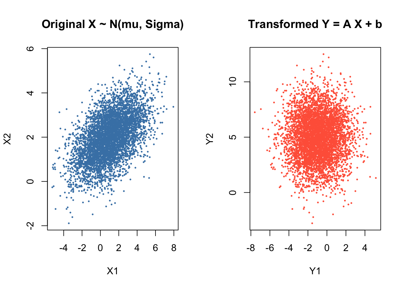
Compare the scatterplots.

set.seed(1234)

library(MASS)

# Original distribution
mu  <- c(1, 2)
Sigma <- matrix(c(4, 1,
                  1, 1), 2, 2)

n <- 5000
X <- mvrnorm(n, mu = mu, Sigma = Sigma)

# Linear transformation
A <- matrix(c(1, 0,
             -1, 2), 2, 2)
b <- c(0, 1)

# Matrix algebra
Y <- t(A %*% t(X)) + matrix(b, n, 2, byrow = TRUE)

par(mfrow = c(1, 2))

plot(X[,1], X[,2], pch = 16, cex = 0.4, col = "steelblue",
     main = "Original X ~ N(mu, Sigma)",
     xlab = "X1", ylab = "X2")

plot(Y[,1], Y[,2], pch = 16, cex = 0.4, col = "tomato",
     main = "Transformed Y = A X + b",
     xlab = "Y1", ylab = "Y2")

The original cloud has a certain tilt and spread.
The transformed cloud is rotated and stretched exactly as predicted by \(A\Sigma A^{\top }\).

23.3 Constructing a Multivariate Normal via Cholesky

If \(\Sigma\) is a covariance matrix, we can write:

\[ \Sigma = LL^\top, \]

where \(L\) is the Cholesky factor (lower triangular).
If \(\mathbf{Z} \sim N(\mathbf{0}, I)\), then

\[ \mathbf{X} = L\mathbf{Z} + \boldsymbol{\mu} \]

has distribution \(N(\boldsymbol{\mu}, \Sigma)\).

This generalises earlier 2D construction:

\[ Y = \rho Z_1 + \sqrt{1-\rho^2}\, Z_2, \]

which is exactly the Cholesky factor of \(\begin{pmatrix}1 & \rho \\ \rho & 1\end{pmatrix}\).

Example: Constructing Correlated Normals via Cholesky

Define the covariance matrix

\[\Sigma =\left( \begin{matrix}1&\rho \\ \rho &1\end{matrix}\right) =\left( \begin{matrix}1&0.8\\ 0.8&1\end{matrix}\right).\]

Both variables \(X\) and \(Y\) have variance 1, and covariance \(\rho\).

set.seed(1234)

n <- 5000
rho <- 0.8

# Covariance matrix
Sigma <- matrix(c(1, rho,
                  rho, 1), 2, 2)

# Cholesky factor: L^T L (upper triangular)
L <- chol(Sigma)

# Generate 2n independent N(0,1) values
Z <- matrix(rnorm(2*n), n, 2)

# Construct X = Z L^T (linear transformation)
X <- Z %*% L

par(mfrow = c(1, 2))

plot(Z[,1], Z[,2], pch = 16, cex = 0.4, col = "gray60",
     main = "Z ~ N(0, I)",
     xlab = "Z1", ylab = "Z2")

plot(X[,1], X[,2], pch = 16, cex = 0.4, col = "firebrick",
     main = "X = Z L^T (Correlated Normals)",
     xlab = "X1", ylab = "X2")

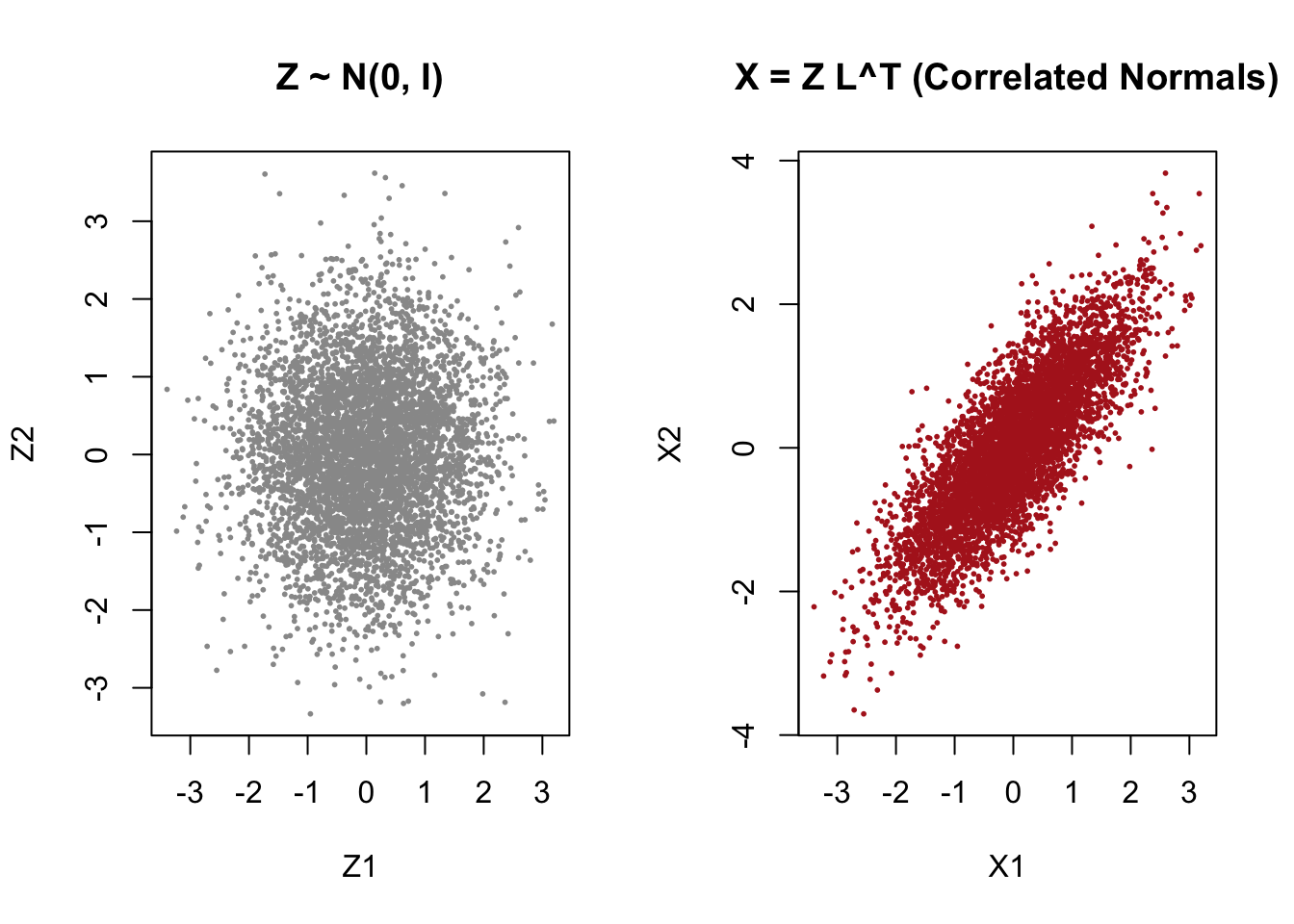
\(Z\) is a round cloud (independent normals).
\(X\) becomes a tilted ellipse with correlation \(\rho =0.8\).
This is how Cholesky induces covariance.

Example: General k‑Dimensional Construction

Simulate \(\mathbf{X}\sim N(\mu ,\Sigma )\) using Cholesky.

Define a mean vector and a covariance matrix:

\[ \mu =(0,\; 1,\; 2)^{\top }, \qquad \Sigma =\left( \begin{matrix}1&0.5&0.2\\ 0.5&2&0.3\\ 0.2&0.3&1\end{matrix}\right). \]

set.seed(1234)

# 3D mean and covariance
mu <- c(0, 1, 2)
Sigma <- matrix(c(1, 0.5, 0.2,
                  0.5, 2, 0.3,
                  0.2, 0.3, 1), 3, 3)

n <- 5000

# Cholesky factor L^T
L <- chol(Sigma)

# Standard normals
Z <- matrix(rnorm(3*n), n, 3)

# Construct X = Z L^T + mu
X <- Z %*% L + matrix(mu, n, 3, byrow = TRUE)

# Quick diagnostic: sample covariance
round(cov(X), 2)

     [,1] [,2] [,3]
[1,] 0.98 0.54 0.21
[2,] 0.54 1.98 0.31
[3,] 0.21 0.31 1.00

The sample covariance of \(X\) matches \(\Sigma\).
The construction works in any dimension.

set.seed(1234)

# 3D mean and covariance
mu <- c(0, 1, 2)
Sigma <- matrix(c(1, 0.5, 0.2,
                  0.5, 2, 0.3,
                  0.2, 0.3, 1), 3, 3)

n <- 5000

# Cholesky factor L^T
L <- chol(Sigma)

# Standard normals
Z <- matrix(rnorm(3*n), n, 3)

# Construct X = Z L^T + mu
X <- Z %*% L + matrix(mu, n, 3, byrow = TRUE)

# 3D scatterplot
library(scatterplot3d)

scatterplot3d(X[,1], X[,2], X[,3],
              pch = 16, cex.symbols = 0.4,
              color = "steelblue",
              main = "3D Scatterplot of Multivariate Normal Sample",
              xlab = "X1", ylab = "X2", zlab = "X3")

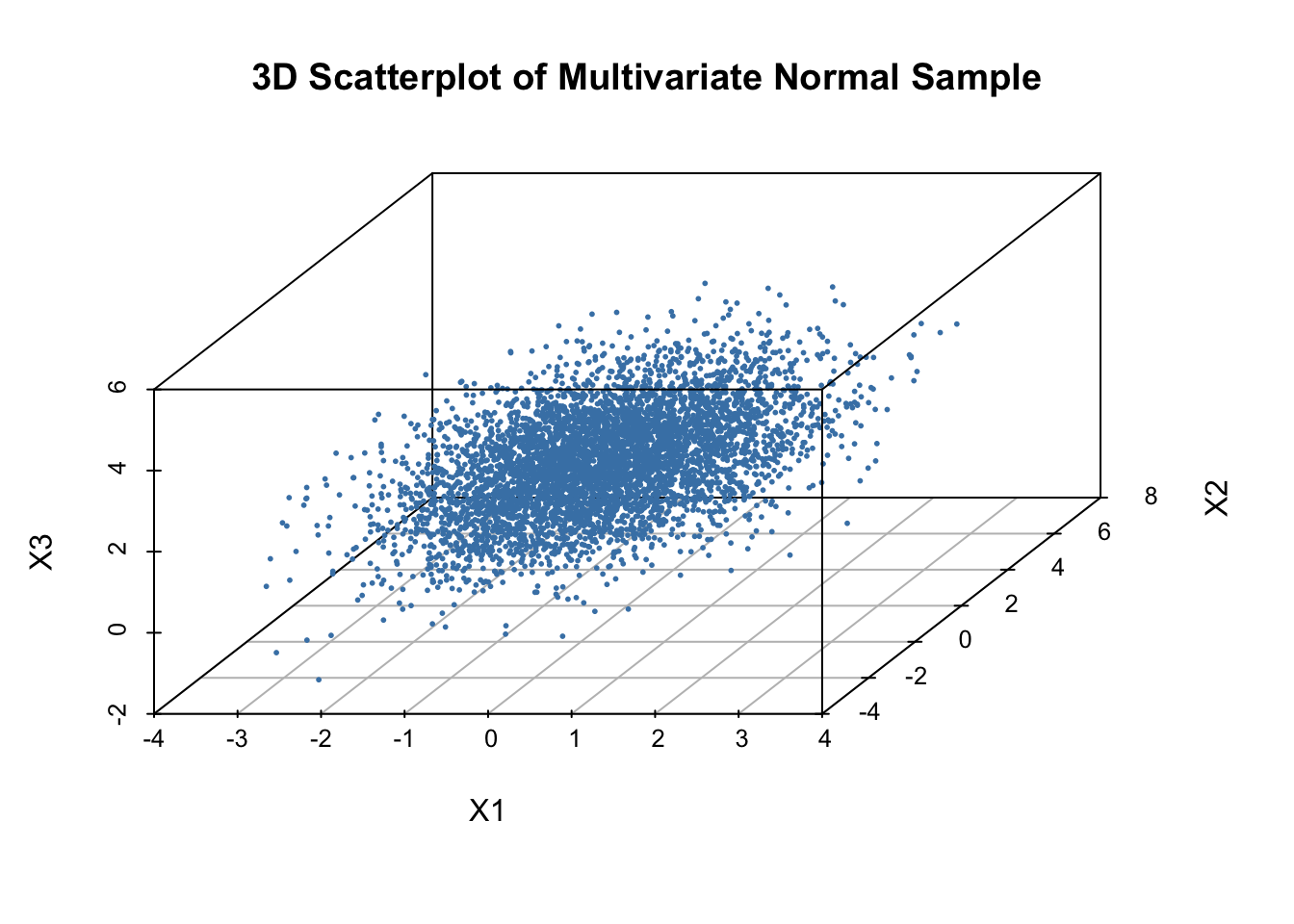
A 3D elliptical cloud whose shape reflects the covariance matrix.
The cloud is tilted and stretched in directions determined by \(\Sigma\).
This visually reinforces the idea that \(X=LZ+\mu\).