37 Vector Autoregressive Model

So far, the AR(1) model has described how a single variable depends on its own past:

\[ X_t = \phi X_{t-1} + \varepsilon_t. \]

This captures memory within one time series. However, many real-world systems involve several variables that evolve together. In such systems, the future value of one variable may depend not only on its own past, but also on the past values of other variables.

For example:

energy demand may depend on past temperature,
stock returns may depend on past interest rates,
infection levels may depend on past mobility patterns,
queue length may depend on past arrival rates and service rates.

To model this kind of interaction, we extend AR(1) to a vector autoregressive model, or VAR.

A simple two-variable VAR(1) model is given by

\[ \begin{aligned} X_t &= a_{11}X_{t-1} + a_{12}Y_{t-1} + \varepsilon_{1,t}, \\ Y_t &= a_{21}X_{t-1} + a_{22}Y_{t-1} + \varepsilon_{2,t}. \end{aligned} \]

\[ \begin{bmatrix} X_t \\ Y_t \end{bmatrix} = \begin{bmatrix} a_{11} & a_{12} \\ a_{21} & a_{22} \end{bmatrix} \begin{bmatrix} X_{t-1} \\ Y_{t-1} \end{bmatrix} + \begin{bmatrix} \varepsilon_{1,t} \\ \varepsilon_{2,t} \end{bmatrix} \]

\[ \mathbf{X}_t = \Phi \mathbf{X}_{t-1} + \boldsymbol{\varepsilon}_t \]

Here:

\(X_t\) and \(Y_t\) are two time series observed over time,
\(a_{11}\) and \(a_{22}\) measure each variable’s dependence on its own past,
\(a_{12}\) and \(a_{21}\) measure cross-variable dependence,
\(\varepsilon_{1,t}\) and \(\varepsilon_{2,t}\) are white noise shocks.

The key idea is simple:

AR(1) models memory within one variable; VAR models memory and interaction across several variables.

Each coefficient describes how information is carried forward through time.

Coefficient	Interpretation
\(a_{11}\)	effect of past \(X\) on current \(X\)
\(a_{22}\)	effect of past \(Y\) on current \(Y\)
\(a_{12}\)	effect of past \(Y\) on current \(X\)
\(a_{21}\)	effect of past \(X\) on current \(Y\)

The diagonal terms (\(a_{11}\) and \(a_{22}\)) describe lagged own-memory (autoregressive effects), similar to \(\phi\) in AR(1).

The off-diagonal terms (\(a_{12}\) and \(a_{21}\)) describe lagged cross-effects, where one variable influences another over time.

For a VAR(1) model to be stable (covariance stationary), the eigenvalues of the coefficient matrix must lie inside the unit circle:

\[ \rho(\Phi) < 1, \]

where \(\rho(\Phi)\) is the spectral radius (largest absolute eigenvalue) of \(\Phi\) calculated as:

\[ \rho(\Phi) = \max_i \{ |\lambda_i| : \lambda \text{ is an eigenvalue of } \Phi \}. \]

Shock Propagation Across Variables

In AR(1), a shock to \(X_t\) can affect future values of \(X\). In VAR, a shock to one variable can spread to other variables.

For example, suppose \(X_t\) receives a large positive shock. Then:

future \(X\) values may be affected through \(a_{11}\),
future \(Y\) values may be affected through \(a_{21}\),
once \(Y\) changes, it may feed back into \(X\) through \(a_{12}\).

This creates a system of dynamic feedback.

VAR models are useful when we want to study how shocks move through an interacting system.

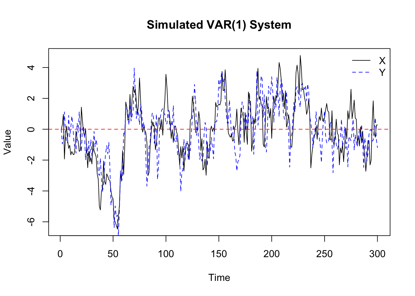
Example: Simulate a simple VAR(1) system:

\[ \begin{aligned} X_t &= 0.6X_{t-1} + 0.3Y_{t-1} + \varepsilon_{1,t}, \\ Y_t &= 0.4X_{t-1} + 0.5Y_{t-1} + \varepsilon_{2,t}. \end{aligned} \]

Here, both variables depend on their own past and on each other’s past.

set.seed(1234)

n <- 300

X <- numeric(n)
Y <- numeric(n)

epsilon_x <- rnorm(n, mean = 0, sd = 1)
epsilon_y <- rnorm(n, mean = 0, sd = 1)

X[1] <- 0
Y[1] <- 0

for (t in 2:n) {
  X[t] <- 0.6 * X[t - 1] + 0.3 * Y[t - 1] + epsilon_x[t]
  Y[t] <- 0.4 * X[t - 1] + 0.5 * Y[t - 1] + epsilon_y[t]
}

plot(
  X,
  type = "l",
  main = "Simulated VAR(1) System",
  xlab = "Time",
  ylab = "Value"
)
lines(Y, lty = 2, col = "blue")
abline(h = 0, col = "red", lty = 2)
legend(
  "topright",
  legend = c("X", "Y"),
  lty = c(1, 2),
  col = c("black", "blue"),
  bty = "n"
)

Python Version

import numpy as np
import matplotlib.pyplot as plt

np.random.seed(1234)

n = 300

X = np.zeros(n)
Y = np.zeros(n)

epsilon_x = np.random.normal(0, 1, n)
epsilon_y = np.random.normal(0, 1, n)

for t in range(1, n):
    X[t] = 0.6 * X[t - 1] + 0.3 * Y[t - 1] + epsilon_x[t]
    Y[t] = 0.4 * X[t - 1] + 0.5 * Y[t - 1] + epsilon_y[t]

plt.plot(X, label="X")
plt.plot(Y, linestyle="--", label="Y")
plt.axhline(0, color="red", linestyle="--")
plt.title("Simulated VAR(1) System")
plt.xlabel("Time")
plt.ylabel("Value")
plt.legend()
plt.show()

In this simulated system:

\(X_t\) depends on past \(X\) and past \(Y\),
\(Y_t\) depends on past \(Y\) and past \(X\),
shocks to one variable can influence the other variable later,
the two series move as an interacting system rather than as isolated processes.

This is the main conceptual leap from AR(1) to VAR.

Isolating a Shock

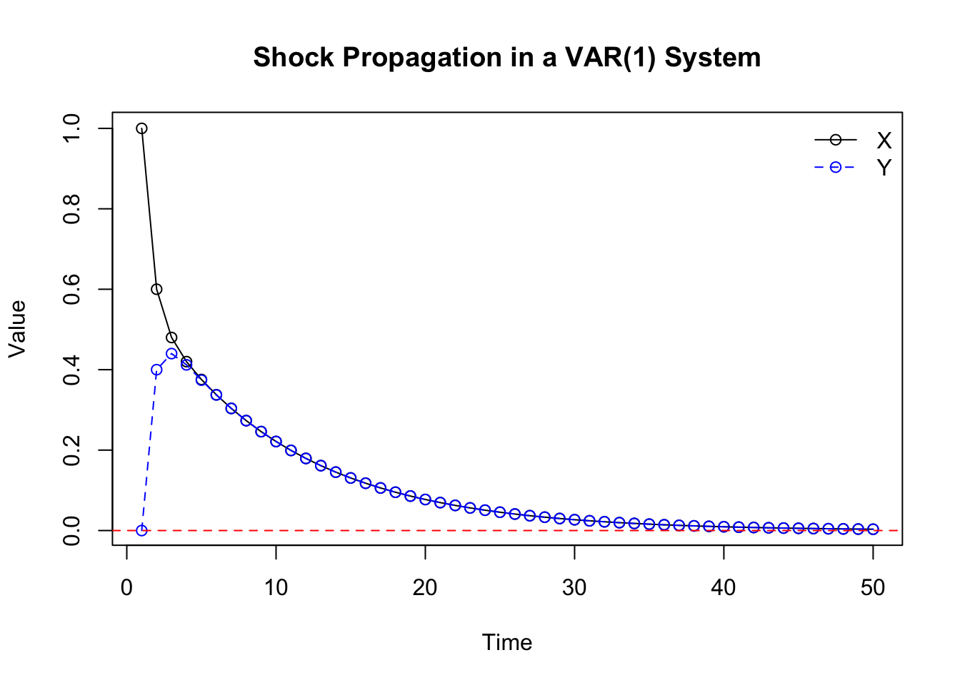
To see cross-variable shock propagation more clearly, we can remove random noise and introduce a one-time shock to \(X\).

Example: A one-time shock to \(X\) propagates through both \(X\) and \(Y\).

n <- 50

X <- numeric(n)
Y <- numeric(n)

X[1] <- 1  # initial shock to X
Y[1] <- 0

for (t in 2:n) {
  X[t] <- 0.6 * X[t - 1] + 0.3 * Y[t - 1]
  Y[t] <- 0.4 * X[t - 1] + 0.5 * Y[t - 1]
}

plot(
  X,
  type = "o",
  main = "Shock Propagation in a VAR(1) System",
  xlab = "Time",
  ylab = "Value"
)
lines(Y, type = "o", lty = 2, col = "blue")
abline(h = 0, col = "red", lty = 2)
legend(
  "topright",
  legend = c("X", "Y"),
  lty = c(1, 2),
  pch = c(1, 1),
  col = c("black", "blue"),
  bty = "n"
)

Python Version

import numpy as np
import matplotlib.pyplot as plt

n = 50

X = np.zeros(n)
Y = np.zeros(n)

X[0] = 1  # initial shock to X
Y[0] = 0

for t in range(1, n):
    X[t] = 0.6 * X[t - 1] + 0.3 * Y[t - 1]
    Y[t] = 0.4 * X[t - 1] + 0.5 * Y[t - 1]

plt.plot(X, marker="o", label="X")
plt.plot(Y, marker="o", linestyle="--", label="Y")
plt.axhline(0, color="red", linestyle="--")
plt.title("Shock Propagation in a VAR(1) System")
plt.xlabel("Time")
plt.ylabel("Value")
plt.legend()
plt.show()

The plot shows that the initial shock directly affects \(X\), but then spreads to \(Y\) through the cross-effect term \(a_{21}\). Once \(Y\) changes, it can also feed back into \(X\) through \(a_{12}\).

Thus, a VAR model allows us to study not only whether shocks persist, but also where they travel.

Comparison: AR(1) vs VAR(1)

Feature	AR(1)	VAR(1)
Number of variables	One	Two or more
Dependence	Own past only	Own past and other variables’ past
Shock propagation	Through time	Through time and across variables
Main idea	Memory	Interaction

VAR extends the AR idea from a single time series to an interacting system of time series.

The same ideas remain central:

memory,
persistence,
shock propagation,
stability,
simulation.

The only difference is that shocks can now move between variables, not just through time within one variable.