51  🌫️ Air Pollution Monitoring

Air pollution is a major environmental and public health concern, particularly in urban areas where emissions from traffic, industry, and weather conditions interact in complex ways. Monitoring pollution levels across multiple locations is essential for understanding spatial patterns, assessing risk, and informing policy decisions.

In practice, pollution measurements at nearby locations are not independent. For example, wind direction, temperature, and regional emission sources can cause pollution levels at different monitoring stations to rise and fall together. As a result, modelling each location separately fails to capture the true joint behaviour of the system.

A natural way to model such data is through a multivariate normal distribution, where each component represents pollution levels at a different site, and the covariance matrix encodes the dependence between locations. This allows us to simulate realistic scenarios in which pollution levels co-vary across space.

In this example, we compare the differences between:

• Frequentist MVN: treat \(\mu\) and \(\Sigma\) as fixed and known
• Bayesian MVN: treat \(\mu\) and \(\Sigma\) as unknown and assign priors

Background

We consider pollution levels (e.g., PM2.5 concentration) measured at three nearby monitoring stations:

• Site A: \(X_1\)
• Site B: \(X_2\)
• Site C: \(X_3\)

Because the sites are geographically close, pollution levels tend to move together due to shared weather conditions, traffic patterns, and regional emission sources. A multivariate normal model provides a natural way to describe this joint behaviour.

We assume that the vector of pollution levels follows a multivariate normal distribution:

\[ \mathbf{X} = (X_1, X_2, X_3)^\top \sim N(\boldsymbol{\mu}, \Sigma), \]

where:

• \(\boldsymbol{\mu}\) represents the average pollution levels at each site,
• \(\Sigma\) represents the covariance structure capturing spatial dependence (how sites move together).

In a Bayesian model:

• \(\boldsymbol{\mu}\) and \(\Sigma\) are unknown
• we simulate from this distribution repeatedly

Our goal is to:

simulate realistic pollution levels across the three sites while preserving both the marginal behaviour and the dependence structure between locations.

To achieve this, we will construct samples from the multivariate normal distribution using Cholesky decomposition, which allows us to transform independent standard normal variables into correlated variables with the desired covariance structure.

Frequentist MVN

In the frequentist version, we assume that the mean vector and covariance matrix are known constants. Our goal is simply to simulate pollution levels that have the required averages and dependence structure.

This is useful when:

• parameters are given from historical estimates,
• we want to generate synthetic data,
• or we want to understand how covariance affects the joint behaviour.

We assume:

\[ \mathbf{X}=(X_1,X_2,X_3)^\top \sim N(\boldsymbol{\mu}, \Sigma), \]

with

\[ \boldsymbol{\mu} = \begin{pmatrix} 20\\ 25\\ 22 \end{pmatrix}, \qquad \Sigma = \begin{pmatrix} 10 & 6 & 4\\ 6 & 12 & 5\\ 4 & 5 & 8 \end{pmatrix}, \]

where

• \(\mu\) gives the average pollution level at each site,
• \(\Sigma\) describes the variability and dependence.

Then, we simulate realistic pollution measurements at the three sites assuming the mean vector and covariance matrix are known. Use Cholesky decomposition to generate correlated samples from the multivariate normal distribution.

set.seed(123)

# Mean vector
mu <- c(20, 25, 22)

# Covariance matrix
Sigma <- matrix(c(10, 6, 4,
                  6, 12, 5,
                  4, 5, 8), 3, 3)

# Cholesky factor
L <- chol(Sigma)

# Simulate standard normals
n <- 5000
Z <- matrix(rnorm(3 * n), n, 3)

# Construct correlated MVN sample
X <- Z %*% L + matrix(mu, n, 3, byrow = TRUE)

# Check results
colMeans(X)

[1] 19.99820 24.98682 22.01486

cov(X)

         [,1]      [,2]     [,3]
[1,] 9.891714  5.880366 3.975450
[2,] 5.880366 11.942226 4.997649
[3,] 3.975450  4.997649 8.024612

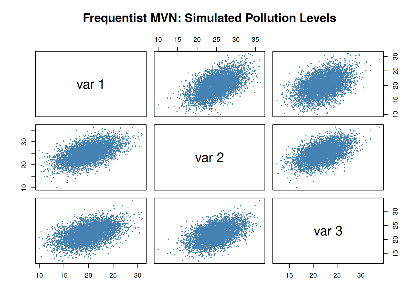
# Pairwise plots
pairs(X, pch = 16, cex = 0.4, col = "steelblue",
      main = "Frequentist MVN: Simulated Pollution Levels")

• Each column represents one monitoring site.
• The sample means should be close to \(\mu\).
• The sample covariance matrix should be close to \(\Sigma\).
• The scatterplots should show positive dependence between sites.

In the frequentist MVN model, the parameters are fixed, and we simulate pollution levels conditional on those values.

Bayesian MVN

In practice, the true mean pollution levels and covariance structure are usually unknown. A Bayesian approach treats these parameters as random variables and updates them using observed data.

This means we account for two layers of uncertainty:

1. uncertainty in the pollution measurements themselves,
2. uncertainty in the unknown parameters \(\mu\) and \(\Sigma\).

We observed pollution vectors

\[ \mathbf{X}_1,\dots,\mathbf{X}_n \mid \mu,\Sigma \sim N(\mu,\Sigma), \]

with both \(\mu\) and \(\Sigma\) are unknown.

Prior (conjugate)

We use the Normal–Inverse‑Wishart prior:

\[ \mu \mid \Sigma \sim N\!\left(\mu_0,\frac{\Sigma}{\kappa_0}\right), \qquad \Sigma \sim \text{Inverse-Wishart}(\Psi_0,\nu_0), \]

where

• \(\mu_0\) is prior mean,
• \(\kappa_0\) is prior strength (pseudo sample size for the mean),
• \(\Psi_0, \nu_0\) are prior scale and degrees of freedom for \(\Sigma\).

Posterior

Let:

• \(\bar{\mathbf X}\) = sample mean
• \(S = \sum_{i=1}^n (\mathbf X_i-\bar{\mathbf X})(\mathbf X_i-\bar{\mathbf X})^\top\)

Then the posterior is:

\[ \Sigma \mid \mathbf X \sim \text{Inv-Wishart}(\Psi_n,\nu_n), \]

\[ \mu \mid \Sigma,\mathbf X \sim N_p\!\left(\mu_n,\frac{\Sigma}{\kappa_n}\right), \]

where

\[ \kappa_n = \kappa_0 + n, \qquad \nu_n = \nu_0 + n, \]

\[ \mu_n = \frac{\kappa_0\mu_0 + n\bar{\mathbf X}}{\kappa_n}, \]

\[ \Psi_n = \Psi_0 + S + \frac{\kappa_0 n}{\kappa_n} (\bar{\mathbf X}-\mu_0)(\bar{\mathbf X}-\mu_0)^\top. \]

Posterior Predictive Distribution (key result)

After integrating out \(\mu\) and \(\Sigma\):

\[ \mathbf{X_{\text{new}}} \mid \mathbf{X} \;\sim\; \text{Multivariate-}t_{\nu_n-p+1} \left( \mu_n,\; \frac{\kappa_n+1}{\kappa_n(\nu_n-p+1)}\Psi_n \right). \]

This is the exact Bayesian predictive distribution.
It has heavier tails than a Gaussian, reflecting parameter uncertainty.

Bayesian Simulation Algorithm

1. Sample \(\Sigma^{(s)} \sim \text{Inv-Wishart}(\Psi_n,\nu_n)\)
2. Sample \(\mu^{(s)} \mid \Sigma^{(s)} \sim N(\mu_n,\Sigma^{(s)}/\kappa_n)\)
3. Sample \(\mathbf X_{\text{new}}^{(s)} \sim N(\mu^{(s)},\Sigma^{(s)})\)
4. Repeat for \(s=1,\dots,S\).

In practice, we do not know the true mean vector or covariance matrix. We only observe data and estimate these quantities using the sample mean and sample covariance. In this example, we simulate data using “true” parameters to illustrate the process, but in real applications these parameters must be inferred from data.

library(MASS)
set.seed(1234)

# Simulate synthetic pollution data
mu_true <- c(20, 25, 22) # unknown in reality
Sigma_true <- matrix(c(10, 6, 4,
                       6, 12, 5,
                       4, 5, 8), 3, 3) # unknown in reality

X_obs <- mvrnorm(100, mu = mu_true, Sigma = Sigma_true)

# In practice, we estimate parameters from the observed data
colMeans(X_obs)

[1] 20.50903 25.24295 22.54921

cov(X_obs)

          [,1]      [,2]     [,3]
[1,] 10.507274  6.049016 3.842170
[2,]  6.049016 12.709741 4.929106
[3,]  3.842170  4.929106 6.930013

# Dimensions
p <- 3
n <- nrow(X_obs)

# Sample statistics
xbar <- colMeans(X_obs)
S <- t(X_obs - xbar) %*% (X_obs - xbar)

# Prior hyperparameters (weakly informative)
mu0 <- c(20, 25, 22)
kappa0 <- 0.01
nu0 <- p + 2
Psi0 <- diag(p)

# Posterior hyperparameters
kappa_n <- kappa0 + n
nu_n <- nu0 + n

mu_n <- (kappa0 * mu0 + n * xbar) / kappa_n

Psi_n <- Psi0 + S +
  (kappa0 * n / kappa_n) * tcrossprod(xbar - mu0)

# Number of posterior predictive draws
n_post <- 1000
X_pred <- matrix(NA, n_post, p)

for (i in 1:n_post) {
  # Sample Sigma | data
  Sigma_draw <- solve(rWishart(1, nu_n, solve(Psi_n))[,,1])

  # Sample mu | Sigma, data
  mu_draw <- mvrnorm(1, mu_n, Sigma_draw / kappa_n)

  # Sample new observation
  X_pred[i, ] <- mvrnorm(1, mu_draw, Sigma_draw)
}

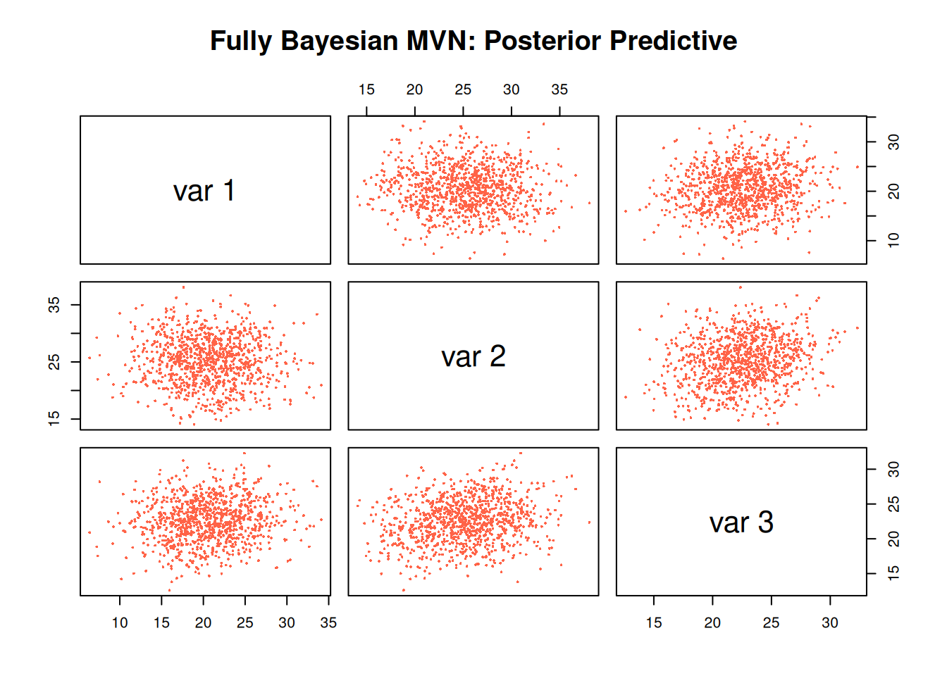
pairs(X_pred, pch = 16, cex = 0.4, col = "tomato",
      main = "Fully Bayesian MVN: Posterior Predictive")

Frequentist MVN

• \(\mu,\Sigma\) fixed
• Variability only from data noise
• Gaussian elliptical clouds

Bayesian MVN

• \(\mu,\Sigma\) both random
• Predictive distribution is multivariate t
• Heavier tails
• More realistic uncertainty
• Correct propagation of parameter uncertainty

Feature	Frequentist MVN	Bayesian MVN
Mean vector \(\mu\)	fixed	random
Covariance matrix \(\Sigma\)	fixed	random
Simulation target	data only	parameters and data
Uncertainty	data variability	data + parameter uncertainty